Basic Analysis
The documentation below describes how to use the code base to analyze output from the U-net model on Animus. This guide assumes you have read through the Installation, Data, and Running the model pages and have model output available for analysis on Animus.
Table of Contents
Before you start
A good thing to do before starting is to check the version of the unox package you are using and the current working directory.
The first time you run a cell in a notebook in VSCodium, it will ask you to select an environment to use.
Be sure to select uplt, or whatever you named the environment during Installation.
import unox
print(unox.__version__)
0.1.1
If this command outputs an error, check where you are trying to run this notebook. By following the Installation, Data, and Running the model pages, this notebook will only run correctly on Animus.
import os
os.getcwd()
'/home/docs/checkouts/readthedocs.org/user_builds/unox/checkouts/stable/docs'
The current working directory for this example guide is within the docs/ directory.
For this reason, most of the file paths below are prepended by ../ to indicate that you must first go up one directory level, then search for the file.
When doing analysis, I generally use a Jupyter Notebook.
The notebook named plot_tests.ipynb is deliberately left blank as a place to test things out.
I encourage you to follow along in that notebook as you go through this guide, noting any differences you need to keep track of based on the working directory and trying out different combinations that aren’t explicitly explored here.
Exploring a dataset
The code base contains a number of methods of exploring a dataset that is in a netCDF file. A number of sample datasets are listed below. Pick one to explore with this section.
# ERA5 U-wind component for 2019
sample_dataset = '../datafiles/sample_data/2019u10.nc'
# `t106` NOx emissions over North America for 2019
# sample_dataset = '../datafiles/sample_data/nox_2019_t106_US.nc'
# TROPESS reanalysis NOx for 2021
# sample_dataset = '../datafiles/sample_data/TROPESS_reanalysis_mon_emi_nox_anth_2021.nc'
# An example input netCDF
# sample_dataset = '../inputfiles/no2_2019_JFM/no2_2019_JFM.nc'
# An example output netCDF
# sample_dataset = '../HPC_runs/no2_example_run/predictions.nc'
Inspecting with Jupyter Notebook output
The simplest way to see what a dataset contains is to load it with xarray:
from xarray import open_dataset

open_dataset(sample_dataset)
<xarray.Dataset> Size: 20MB
Dimensions:     (valid_time: 365, latitude: 56, longitude: 120)
Coordinates:
    number      int64 8B ...
  * latitude    (latitude) float32 224B 11.78 12.9 14.02 ... 71.21 72.34 73.46
  * longitude   (longitude) float32 480B -174.4 -173.2 -172.1 ... -41.62 -40.5
  * valid_time  (valid_time) datetime64[ns] 3kB 2019-01-01 ... 2019-12-31
Data variables:
    u10         (valid_time, latitude, longitude) float64 20MB ...
Attributes:
    GRIB_centre:             ecmf
    GRIB_centreDescription:  European Centre for Medium-Range Weather Forecasts
    GRIB_subCentre:          0
    Conventions:             CF-1.7
    institution:             European Centre for Medium-Range Weather Forecasts
history: 2025-02-07T19:10 GRIB to CDM+CF via cfgrib-0.9.1...The result is an interactive output window which can be extremely handy to quickly verify certain aspects of a dataset. The sections that appear will depend on what dataset you are looking at, but generally include:
Dimensions
The names and lengths of the dimensions of the dataset.
Coordinates
The arrays which define the values of the dimensional axes.
Data variables
The arrays of values for each data variable.
Indexes
The coordinate arrays which are used to index data locations in the dataset.
Attributes
Metadata about the dataset (i.e., data sources, creation date, attributions, formatting notes, etc.)
The dimensions, coordinates, and indexes for a dataset are interrelated.
While the specific distinctions between them do matter in particular cases, generally they define the axes across which the data is stored.
See the xarray Terminology page for details.
In the output above, there are several interactive features:
Arrows next to sections (far left)
Click these to expand or collapse each section.
Metadata (symbol that looks like a file, far right)
Click these to see a particular aspect’s metadata (i.e., long name, units, etc.).
Data preview (symbol that looks like a cylinder, far right)
Click these to see a preview of the data stored in a particular aspect.
Inspecting with map plots
While viewing the interactive text-based output above can give you a quick overview of what is in a dataset, it is often helpful to see plots of the data.
NASA provides an application called Panoply which is a powerful tool for visualizing netCDF files containing geospatial data.
If you are familiar with Panoply, please feel free to use it.
Otherwise, the code base of unox includes several plotting functions which can quickly give an idea of what the dataset contains.
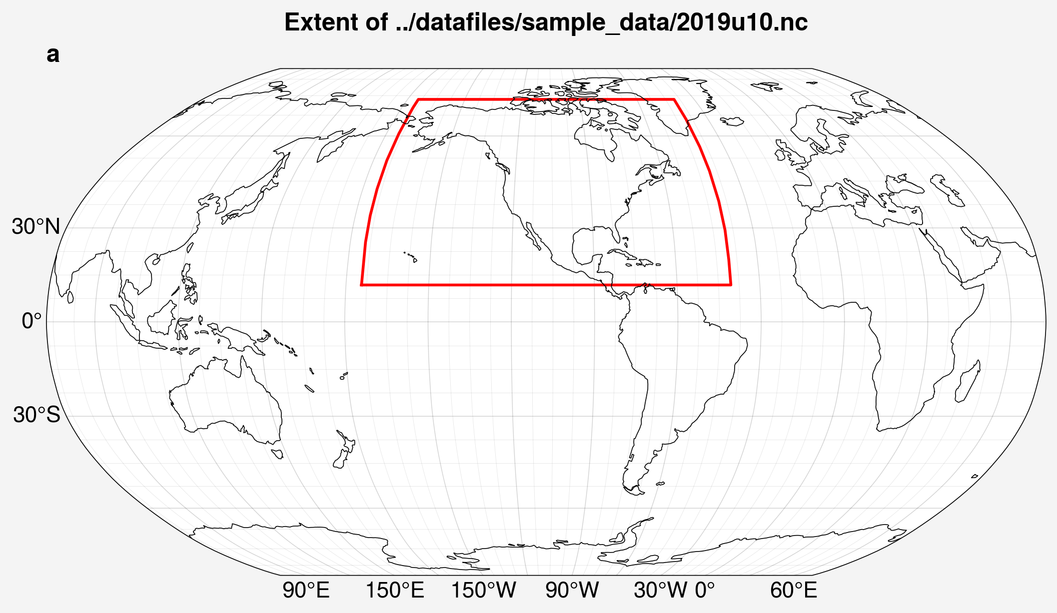
The cell below shows the use of a function to simply plot a box on a world map showing the maximum and minimum extents of the dataset in latitude and longitude.
from unox.plotting import plot_extent

extent_plot = plot_extent(sample_dataset)
Matplotlib is building the font cache; this may take a moment.
/home/docs/checkouts/readthedocs.org/user_builds/unox/envs/stable/lib/python3.9/site-packages/proplot/__init__.py:6: UserWarning: pkg_resources is deprecated as an API. See https://setuptools.pypa.io/en/latest/pkg_resources.html. The pkg_resources package is slated for removal as early as 2025-11-30. Refrain from using this package or pin to Setuptools<81.
  import pkg_resources as pkg
/home/docs/checkouts/readthedocs.org/user_builds/unox/envs/stable/lib/python3.9/site-packages/proplot/__init__.py:71: ProplotWarning: Rebuilding font cache. This usually happens after installing or updating proplot.
  register_fonts(default=True)
/home/docs/checkouts/readthedocs.org/user_builds/unox/envs/stable/lib/python3.9/site-packages/cartopy/mpl/geoaxes.py:403: UserWarning: The `map_projection` keyword argument is deprecated, use `projection` to instantiate a GeoAxes instead.
  warnings.warn("The `map_projection` keyword argument is "
/home/docs/checkouts/readthedocs.org/user_builds/unox/envs/stable/lib/python3.9/site-packages/cartopy/io/__init__.py:241: DownloadWarning: Downloading: https://naturalearth.s3.amazonaws.com/110m_physical/ne_110m_coastline.zip
  warnings.warn(f'Downloading: {url}', DownloadWarning)
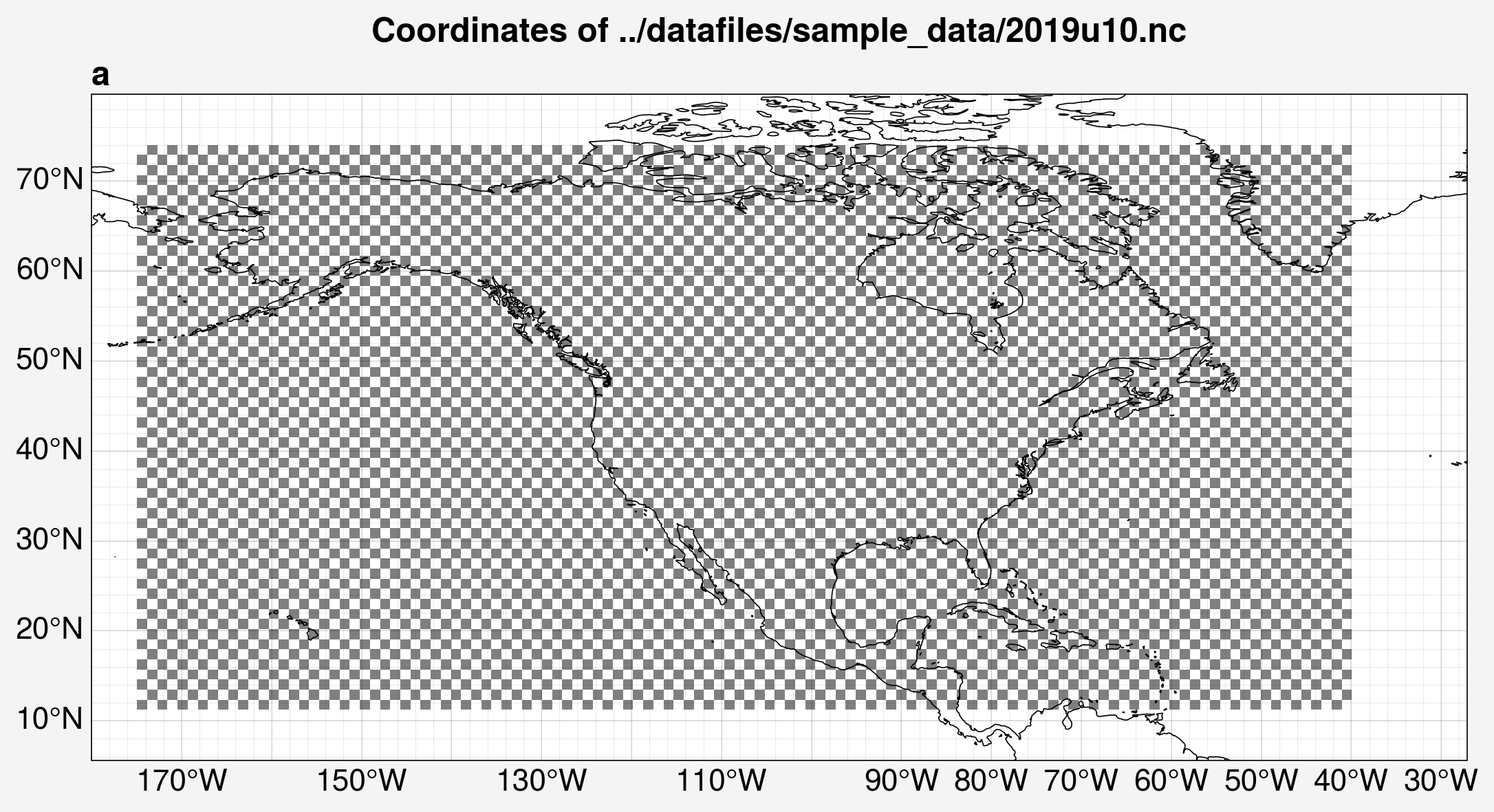
The next cell shows a function which plots a checkered grid on a map to show the rough resolution of the dataset.
You can pass an optional keyword argument padding to change how much space is added around the extent of the dataset.
Note that this function is not currently optimized for datasets that cover the entire globe.
from unox.plotting import plot_lats_lons

lats_lons_plot = plot_lats_lons(sample_dataset)
/home/docs/checkouts/readthedocs.org/user_builds/unox/envs/stable/lib/python3.9/site-packages/cartopy/mpl/geoaxes.py:403: UserWarning: The `map_projection` keyword argument is deprecated, use `projection` to instantiate a GeoAxes instead.
  warnings.warn("The `map_projection` keyword argument is "
/home/docs/checkouts/readthedocs.org/user_builds/unox/envs/stable/lib/python3.9/site-packages/cartopy/io/__init__.py:241: DownloadWarning: Downloading: https://naturalearth.s3.amazonaws.com/50m_physical/ne_50m_coastline.zip
  warnings.warn(f'Downloading: {url}', DownloadWarning)
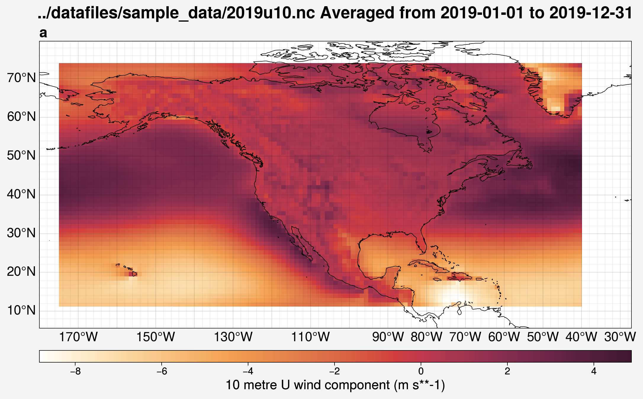
The next few cells show examples of plotting the contents of particular variables from a dataset on a map.
The specific variables (vars), which can be a list, will need to be selected such that they are within the given dataset. By default, the variables are averaged over the full time series.
from unox.plotting import plot_var_maps

var_plots = plot_var_maps(
    '../datafiles/sample_data/2019u10.nc',
    vars = 'u10',
)
/home/docs/checkouts/readthedocs.org/user_builds/unox/checkouts/stable/src/unox/HPC/data0/dataset.py:474: UserWarning: (is_ensemble) `dataset` must be a prediction set to check for ensemble members.
  warnings.warn(f"(is_ensemble) `dataset` must be a prediction set to check for ensemble members.")
/home/docs/checkouts/readthedocs.org/user_builds/unox/envs/stable/lib/python3.9/site-packages/cartopy/mpl/geoaxes.py:403: UserWarning: The `map_projection` keyword argument is deprecated, use `projection` to instantiate a GeoAxes instead.
  warnings.warn("The `map_projection` keyword argument is "
This function also has an optional argument called interval which, if given, will plot the temporal average across the specified time interval to average over starting at the start_date date.
If start_date is not given, it will default to the first datetime in the dataset.
The interval is specified by a string in the format XT where X is an integer and T is the time unit, either D for days or M for months.
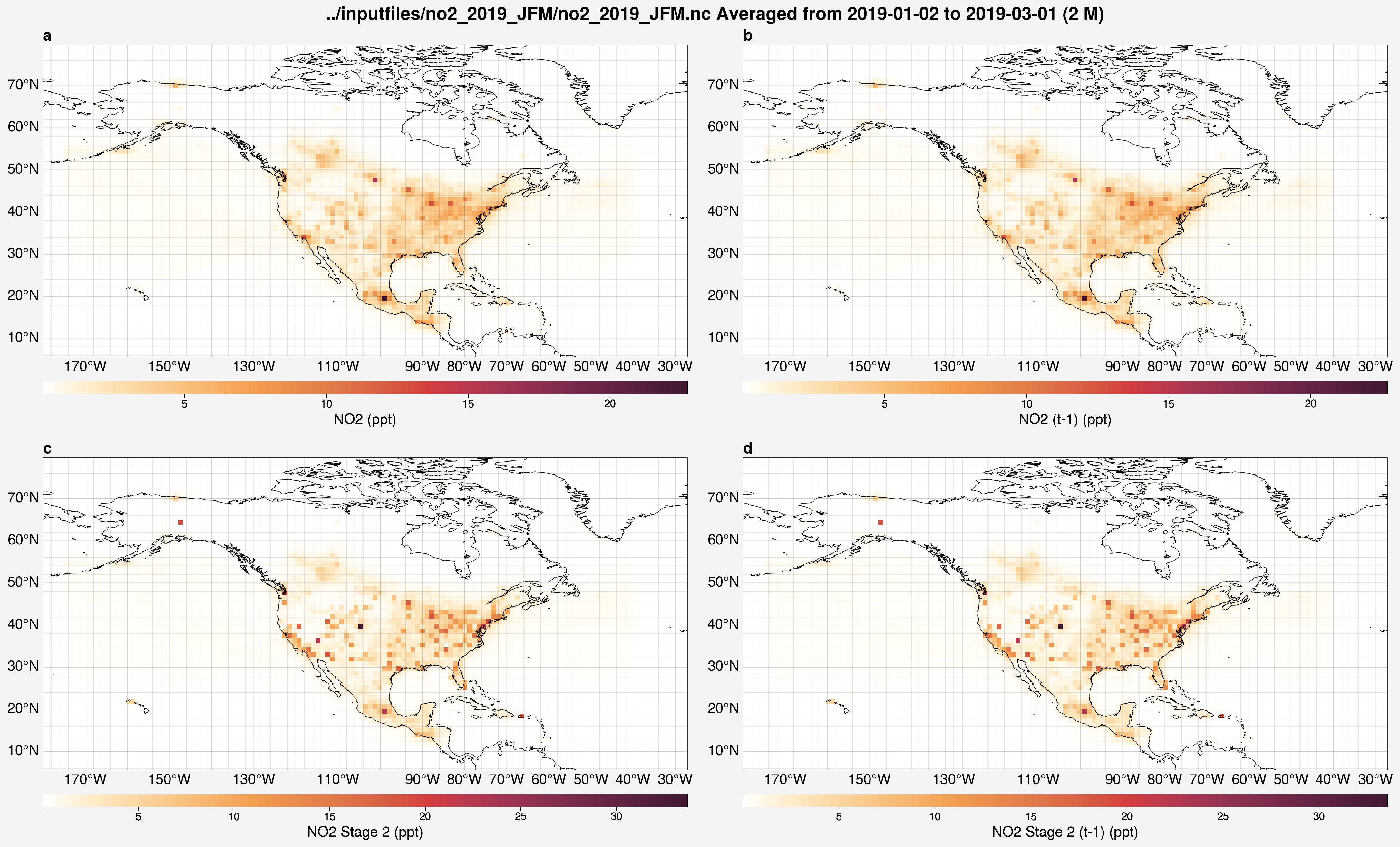
from unox.plotting import plot_var_maps

var_plots = plot_var_maps(
    '../inputfiles/no2_2019_JFM/no2_2019_JFM.nc',
    vars = ['no2', 'no2_tm1', 'no2_s2', 'no2_s2_tm1'],
    start_date='2019-01-01',
    interval='2M',
)
/home/docs/checkouts/readthedocs.org/user_builds/unox/checkouts/stable/src/unox/HPC/data0/dataset.py:474: UserWarning: (is_ensemble) `dataset` must be a prediction set to check for ensemble members.
  warnings.warn(f"(is_ensemble) `dataset` must be a prediction set to check for ensemble members.")
/home/docs/checkouts/readthedocs.org/user_builds/unox/envs/stable/lib/python3.9/site-packages/cartopy/mpl/geoaxes.py:403: UserWarning: The `map_projection` keyword argument is deprecated, use `projection` to instantiate a GeoAxes instead.
  warnings.warn("The `map_projection` keyword argument is "
/home/docs/checkouts/readthedocs.org/user_builds/unox/envs/stable/lib/python3.9/site-packages/cartopy/mpl/geoaxes.py:403: UserWarning: The `map_projection` keyword argument is deprecated, use `projection` to instantiate a GeoAxes instead.
  warnings.warn("The `map_projection` keyword argument is "
/home/docs/checkouts/readthedocs.org/user_builds/unox/envs/stable/lib/python3.9/site-packages/cartopy/mpl/geoaxes.py:403: UserWarning: The `map_projection` keyword argument is deprecated, use `projection` to instantiate a GeoAxes instead.
  warnings.warn("The `map_projection` keyword argument is "
/home/docs/checkouts/readthedocs.org/user_builds/unox/envs/stable/lib/python3.9/site-packages/cartopy/mpl/geoaxes.py:403: UserWarning: The `map_projection` keyword argument is deprecated, use `projection` to instantiate a GeoAxes instead.
  warnings.warn("The `map_projection` keyword argument is "
Inspecting uarray objects
The code base contains an object class called uarray, which is defined in the unox.HPC.data0.dataset module.
This class is meant to extend the functionality of xarray objects by adding custom attributes.
Most of the analysis functions use uarray objects.
The following arguments can be specified when creating a uarray object:
datasetThe only required argument. This is the dataset to make into a
uarrayobject.This can either be an
xarrayobject or a string specifying where the data is located.
is_input_setA boolean option whether the data to add to the
uarrayis an input file.If
True, thendatasetcan simply be a string of the name of the input file and the code will find it in theinputfiles/directory automatically.
is_predictA boolean option whether the data to add to the
uarrayis from a model output prediction.If
True, thendatasetcan simply be a string of the name of the model run and the code will find it in theHPC_runs/directory automatically.
Below is an example of making a uarray from an input file and inspecting the underlying xarray by calling the .xr attribute.
from unox.HPC.data0.dataset import uarray

input_u_arr = uarray('no2_2019_JFM', is_input_set=True)
input_u_arr.xr
<xarray.Dataset> Size: 62MB
Dimensions:     (time: 89, lat: 56, lon: 120, var: 1)
Coordinates:
  * lat         (lat) float32 224B 11.78 12.9 14.02 15.14 ... 71.21 72.34 73.46
  * lon         (lon) float32 480B -174.4 -173.2 -172.1 ... -42.75 -41.62 -40.5
  * time        (time) object 712B 2019-01-02 00:00:00 ... 2019-03-31 00:00:00
Dimensions without coordinates: var
Data variables: (12/13)
    nox         (time, lat, lon, var) float64 5MB ...
    no2         (time, lat, lon) float64 5MB ...
    no2_s2      (time, lat, lon) float64 5MB ...
    no2_tm1     (time, lat, lon) float64 5MB ...
    no2_s2_tm1  (time, lat, lon) float64 5MB ...
    u10         (time, lat, lon) float64 5MB ...
    ...          ...
    blh         (time, lat, lon) float64 5MB ...
    sp          (time, lat, lon) float64 5MB ...
    skt         (time, lat, lon) float64 5MB ...
    t2m         (time, lat, lon) float64 5MB ...
    ssrd        (time, lat, lon) float64 5MB ...
    lsm         (time, lat, lon) float64 5MB ...
Attributes: (12/17)
    description:        Input data for the Unet model. Data for each year is ...
    y_var:              nox
    emiss_dir:          /data/high_res/emacdonald/unet/datafiles/t106
    emiss_pre:          nox_
    emiss_post:         _t106_US.nc
    nan_fill:           0
    ...                 ...
    x2_vars:            ['no2_s2', 'no2_s2_tm1', 'u10', 'v10', 'blh', 'sp', '...
    data_dir:           /data/high_res
    chemra_path:        emacdonald/unet/datafiles/TROPESS/TROPESS_reanalysis_...
    insitu_path:        US_EPA/NO2/daily_NO2/daily_42602_
    era5_path:          ERA5concatenated
stages: [1 2]Below is an example of making a uarray from model predictions and inspecting the underlying xarray by calling the .xr attribute.
from unox.HPC.data0.dataset import uarray

predict_u_arr = uarray('no2_example_run', is_predict=True)
predict_u_arr.xr
<xarray.Dataset> Size: 39MB
Dimensions:      (time: 728, lat: 56, lon: 120)
Coordinates:
  * time         (time) object 6kB 2019-01-02 00:00:00 ... 2020-12-31 00:00:00
  * lat          (lat) float32 224B 11.78 12.9 14.02 15.14 ... 71.21 72.34 73.46
  * lon          (lon) float32 480B -174.4 -173.2 -172.1 ... -42.75 -41.62 -40.5
Data variables:
    nox_pred     (time, lat, lon) float32 20MB ...
    nox_pred_s2  (time, lat, lon) float32 20MB ...
Attributes: (12/18)
    description:        Predicted Surface NOx emissions using a U-net model
    modification_date:  2026-04-10 14:46:06
    y_var:              nox
    input_set:          no2_2005-2020
    config_path:        HPC_runs/no2_example_run/input_config.json
    config_dict:        {'input_set': 'no2_2005-2020', 'x_vars': ['no2', 'no2...
    ...                 ...
    x_vars:             ['no2', 'no2_tm1', 'u10', 'v10', 'blh', 'sp', 'skt', ...
    data_dir:           /data/high_res
    chemra_path:        emacdonald/unet/datafiles/TROPESS/TROPESS_reanalysis_...
    insitu_path:        US_EPA/NO2/daily_NO2/daily_42602_
    era5_path:          ERA5concatenated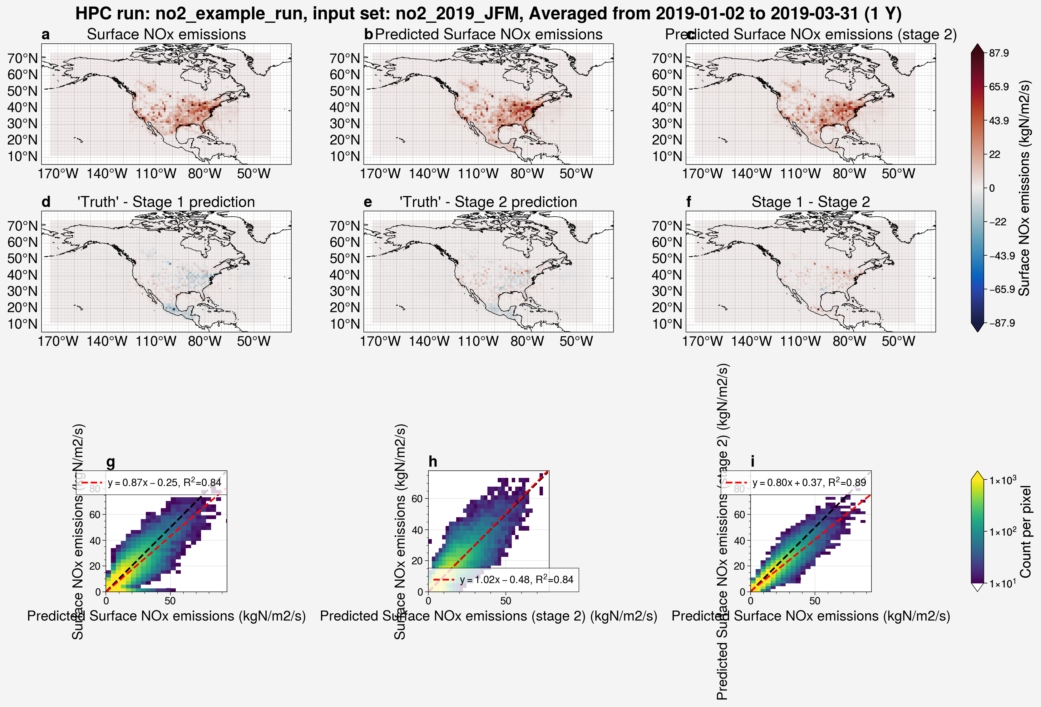
stages: [1 2]The is_input_set and is_predict keyword arguments can be passed to plotting functions to avoid needing to specify the exact file path to the data to plot.
from unox.plotting import plot_var_maps

var_plots = plot_var_maps(
    'no2_example_run',
    is_predict=True,
    vars = ['nox_pred', 'nox_pred_s2'],
    interval='1Y',
)
/home/docs/checkouts/readthedocs.org/user_builds/unox/envs/stable/lib/python3.9/site-packages/cartopy/mpl/geoaxes.py:403: UserWarning: The `map_projection` keyword argument is deprecated, use `projection` to instantiate a GeoAxes instead.
  warnings.warn("The `map_projection` keyword argument is "
/home/docs/checkouts/readthedocs.org/user_builds/unox/envs/stable/lib/python3.9/site-packages/cartopy/mpl/geoaxes.py:403: UserWarning: The `map_projection` keyword argument is deprecated, use `projection` to instantiate a GeoAxes instead.
  warnings.warn("The `map_projection` keyword argument is "
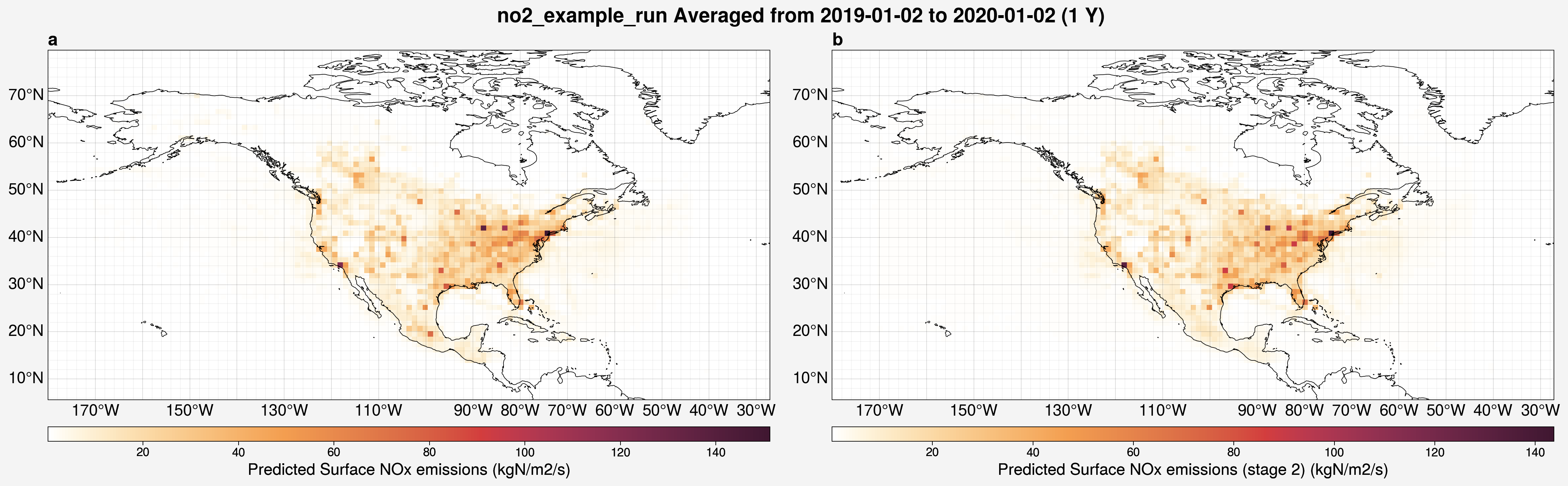
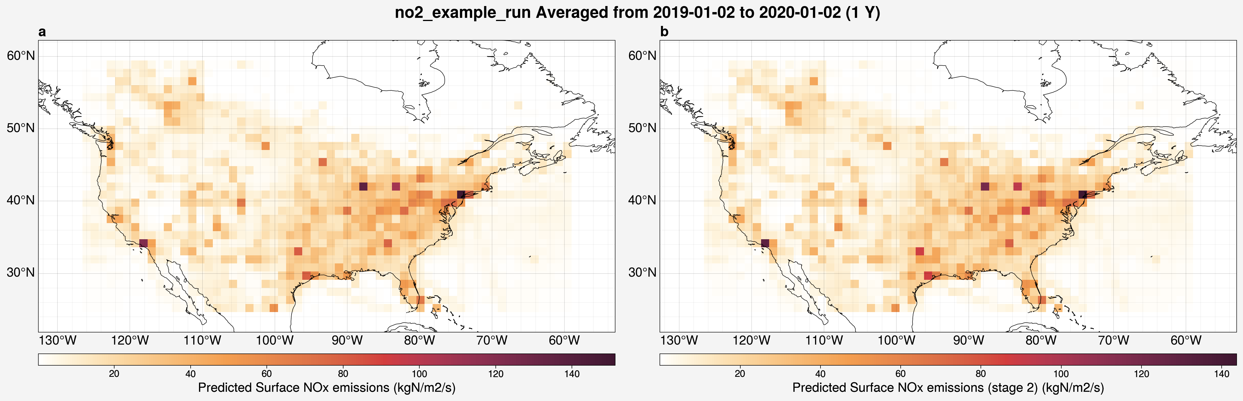
In these maps of the predictions from a model run, edge effects can be clearly seen at the borders of the model domain.
To view the fit without those artifacts, the domain can be restricted to match that of a different dataset, for example, the t106 NOx emissions over North America:
from unox.plotting import plot_var_maps

var_plots = plot_var_maps(
    'no2_example_run',
    is_predict=True,
    vars = ['nox_pred', 'nox_pred_s2'],
    interval='1Y',
    restrict_lat_lon_to='../datafiles/sample_data/nox_2019_t106_US.nc',
)
/home/docs/checkouts/readthedocs.org/user_builds/unox/envs/stable/lib/python3.9/site-packages/cartopy/mpl/geoaxes.py:403: UserWarning: The `map_projection` keyword argument is deprecated, use `projection` to instantiate a GeoAxes instead.
  warnings.warn("The `map_projection` keyword argument is "
/home/docs/checkouts/readthedocs.org/user_builds/unox/envs/stable/lib/python3.9/site-packages/cartopy/mpl/geoaxes.py:403: UserWarning: The `map_projection` keyword argument is deprecated, use `projection` to instantiate a GeoAxes instead.
  warnings.warn("The `map_projection` keyword argument is "
Comparing inputs
If you are generating new input files and would like to compare them to previous iterations, the plotting.compare_input_vars() function might be useful.
In this function, you can specify two arrays to compare to each other by specifying:
input_setThe name of the input file to use.
yearThe year for which to make the comparison.
varThe variable for which to make the comparison.
The function will let you know how many values differ between the two specified arrays and, if there are differences, it will make plots to give an idea of what the differences are.
This was designed to compare two different input files, however the examples below will make comparisons between parts of the same input file for demonstration. First, if the two arrays are exactly equal:
from unox.plotting import compare_input_vars

input_comparison = compare_input_vars(
    {
        'input_set': 'no2_2019_JFM',
        'year': 2019,
        'var': 'no2',
    },
    {
        'input_set': 'no2_2019_JFM',
        'year': 2019,
        'var': 'no2',
    }
)
Shape of no2 from no2_2019_JFM: (89, 56, 120)
Shape of no2 from no2_2019_JFM: (89, 56, 120)
Match found for no2_2019_JFM-2019-no2 vs no2_2019_JFM-2019-no2.
If the arrays do have differences, a figure with 6 plots will be made. In these plots, the first array specified will be labeled as “A” and the second, “B”.
from unox.plotting import compare_input_vars

input_comparison = compare_input_vars(
    {
        'input_set': 'no2_2019_JFM',
        'year': 2019,
        'var': 'no2',
    },
    {
        'input_set': 'no2_2019_JFM',
        'year': 2019,
        'var': 'no2_s2',
    },
    # restrict_lat_lon_to='../datafiles/sample_data/nox_2019_t106_US.nc',
)
Shape of no2 from no2_2019_JFM: (89, 56, 120)
Shape of no2_s2 from no2_2019_JFM: (89, 56, 120)
The input files differ more than the tolerance of 2e-05
Number of differences: 15729 / 598080 ( 2.629915730337079 % )
/home/docs/checkouts/readthedocs.org/user_builds/unox/envs/stable/lib/python3.9/site-packages/cartopy/mpl/geoaxes.py:403: UserWarning: The `map_projection` keyword argument is deprecated, use `projection` to instantiate a GeoAxes instead.
  warnings.warn("The `map_projection` keyword argument is "
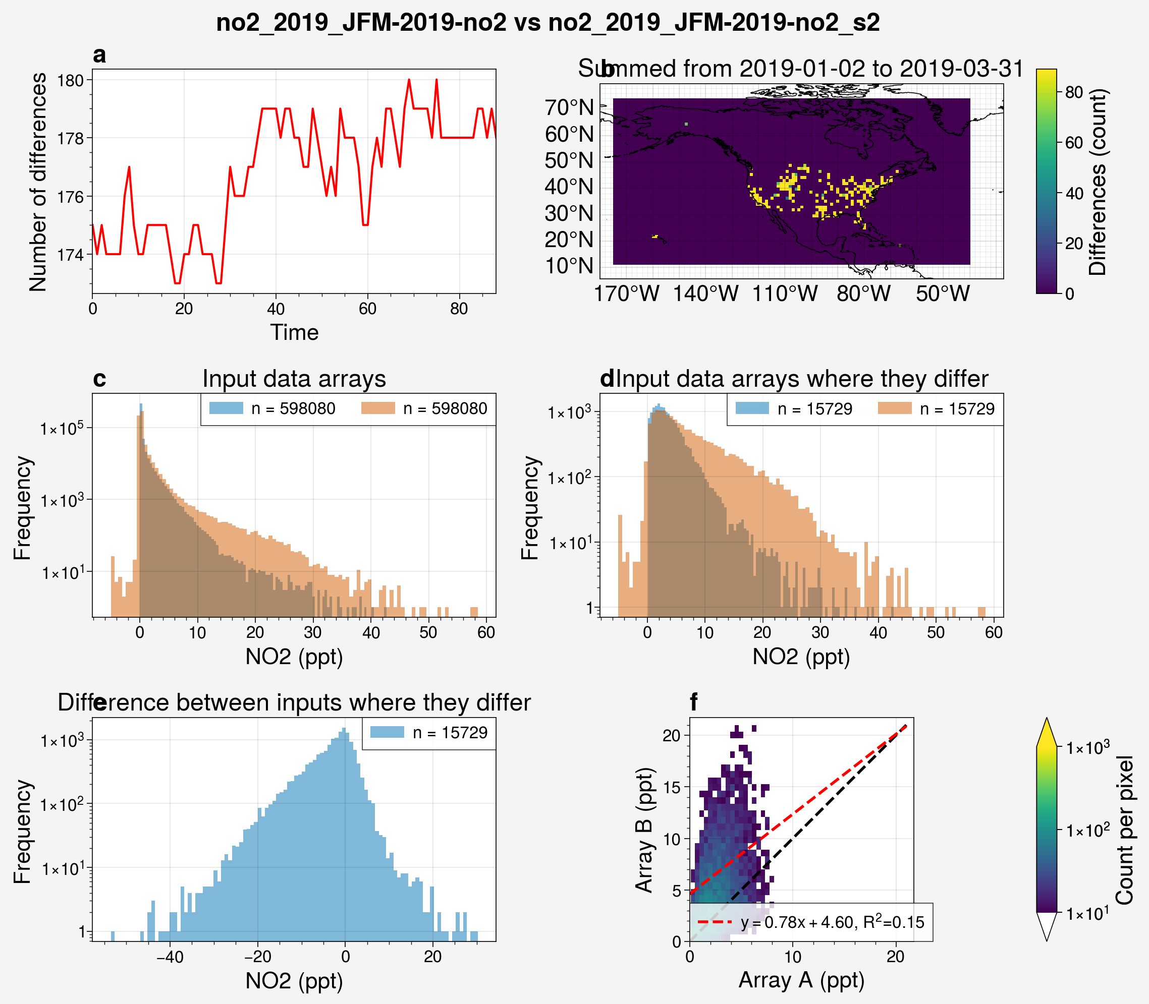
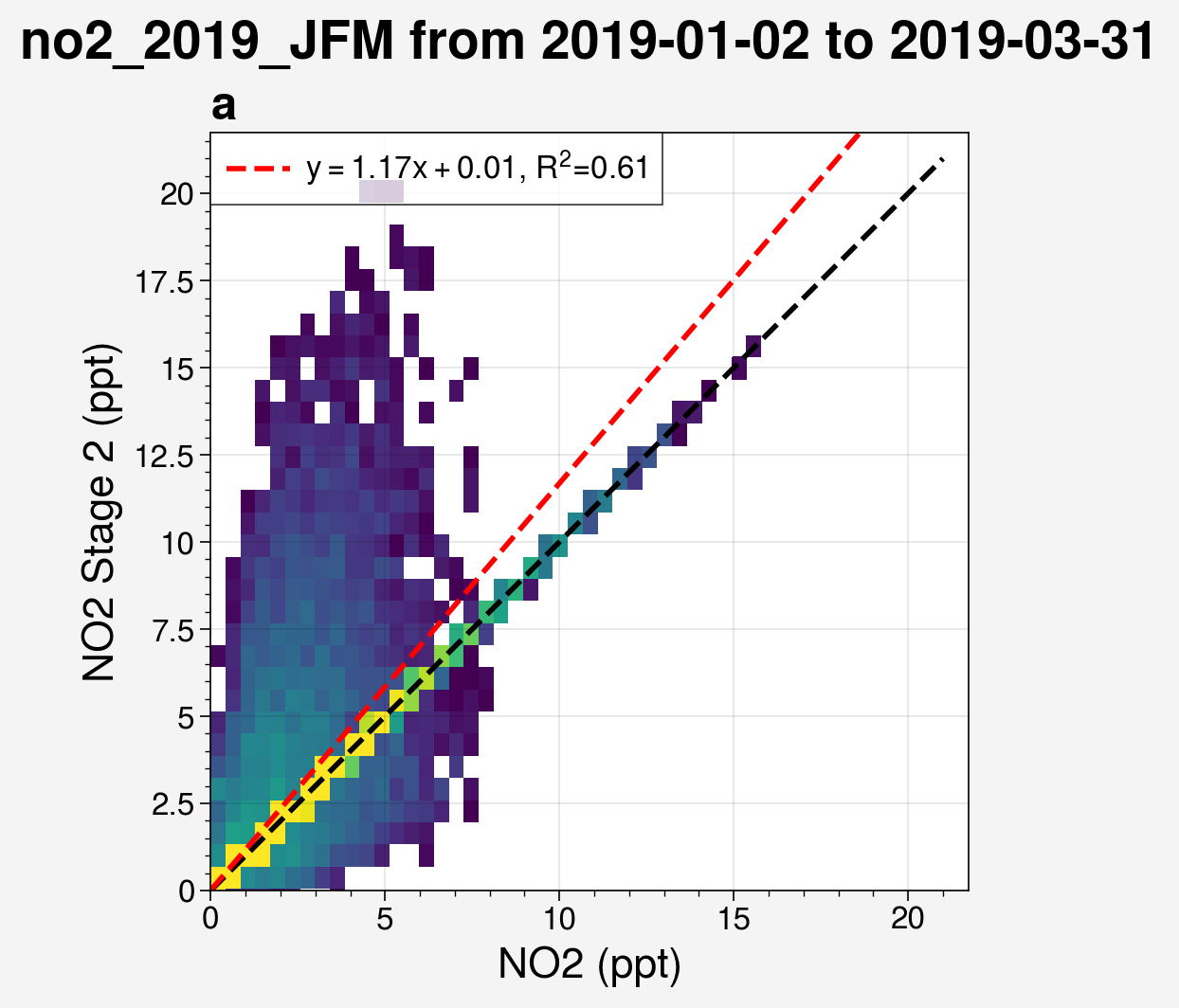
Notably, the last subplot, which shows the correlation, only uses the data where the two arrays differ.
Below is the correlation plot of the full arrays, where a significant number of data points are along the y=x diagonal.
from unox.plotting import corr_plot

this_plt = corr_plot(
    'no2_2019_JFM',
    is_input_set=True,
    x_vars = 'no2',
    y_vars = 'no2_s2',
)
/home/docs/checkouts/readthedocs.org/user_builds/unox/checkouts/stable/src/unox/HPC/data0/dataset.py:474: UserWarning: (is_ensemble) `dataset` must be a prediction set to check for ensemble members.
  warnings.warn(f"(is_ensemble) `dataset` must be a prediction set to check for ensemble members.")
Plotting results
To quickly visualize the results of a model run, use the plot_run_analysis() function.
Generally, that would involve a call like the one below.
from unox.plotting import plot_run_analysis

this_plt = plot_run_analysis(
    'no2_example_run',
)
However, the model run no2_example_run, which is included in this repository, was created using an input file called no2_2005-2020.nc.
That file is large (3.8 GB) and therefore was not included.
If you have followed the Data guide and generated the no2_2005-2020.nc input file in your own instance of the repository, you should be able to copy the above code and run it.
For demonstration purposes, the cell below modifies the no2_example_run dataset such that it can act as if it uses the no2_2019_JFM.nc input file.
The no2_2019_JFM.nc file, which has been used in above examples, is exactly the same as no2_2005-2020.nc, however has been truncated to only include dates between 2019-01-01 and 2019-03-31 to reduce it’s file size to 60 MB.
from unox.HPC.data0.dataset import uarray

no2_ex_uarr = uarray('no2_example_run', is_predict=True)
# Modifying the `no2_example_run` dataset such that it can use `no2_2019_JFM` as the input set for plotting functions instead of `no2_2005-2020`, which is too large to include in the repository. This is just for the purpose of demonstrating the plotting functions with a smaller dataset.
no2_ex_uarr.xr.attrs['input_set'] = 'no2_2019_JFM'
no2_ex_uarr._get_metadata()
no2_ex_uarr.metadata['config_dict']['input_set'] = 'no2_2019_JFM'
no2_ex_uarr.xr = no2_ex_uarr.xr.sel(time=slice("2019-01-01", "2019-03-31"))
from unox.plotting import plot_run_analysis

this_plt = plot_run_analysis(
    no2_ex_uarr,
)
/home/docs/checkouts/readthedocs.org/user_builds/unox/envs/stable/lib/python3.9/site-packages/cartopy/mpl/geoaxes.py:403: UserWarning: The `map_projection` keyword argument is deprecated, use `projection` to instantiate a GeoAxes instead.
  warnings.warn("The `map_projection` keyword argument is "
/home/docs/checkouts/readthedocs.org/user_builds/unox/envs/stable/lib/python3.9/site-packages/cartopy/mpl/geoaxes.py:403: UserWarning: The `map_projection` keyword argument is deprecated, use `projection` to instantiate a GeoAxes instead.
  warnings.warn("The `map_projection` keyword argument is "
/home/docs/checkouts/readthedocs.org/user_builds/unox/envs/stable/lib/python3.9/site-packages/cartopy/mpl/geoaxes.py:403: UserWarning: The `map_projection` keyword argument is deprecated, use `projection` to instantiate a GeoAxes instead.
  warnings.warn("The `map_projection` keyword argument is "
/home/docs/checkouts/readthedocs.org/user_builds/unox/envs/stable/lib/python3.9/site-packages/cartopy/mpl/geoaxes.py:403: UserWarning: The `map_projection` keyword argument is deprecated, use `projection` to instantiate a GeoAxes instead.
  warnings.warn("The `map_projection` keyword argument is "
/home/docs/checkouts/readthedocs.org/user_builds/unox/envs/stable/lib/python3.9/site-packages/cartopy/mpl/geoaxes.py:403: UserWarning: The `map_projection` keyword argument is deprecated, use `projection` to instantiate a GeoAxes instead.
  warnings.warn("The `map_projection` keyword argument is "
/home/docs/checkouts/readthedocs.org/user_builds/unox/envs/stable/lib/python3.9/site-packages/cartopy/mpl/geoaxes.py:403: UserWarning: The `map_projection` keyword argument is deprecated, use `projection` to instantiate a GeoAxes instead.
  warnings.warn("The `map_projection` keyword argument is "
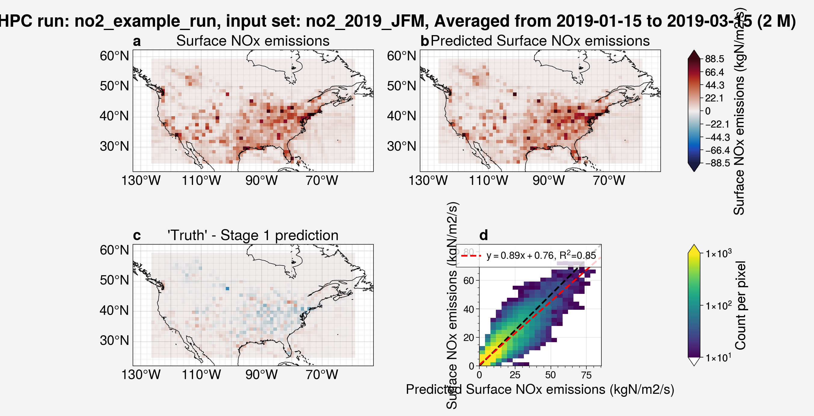
Similar to the functions shown above, there are many arguments which can be added to adjust this plot.
from unox.plotting import plot_run_analysis

this_plt = plot_run_analysis(
    no2_ex_uarr,
    start_date='2019-01-15',
    interval='2M',
    restrict_lat_lon_to='../datafiles/sample_data/nox_2019_t106_US.nc',
    stage1_only=True,
)
/home/docs/checkouts/readthedocs.org/user_builds/unox/envs/stable/lib/python3.9/site-packages/cartopy/mpl/geoaxes.py:403: UserWarning: The `map_projection` keyword argument is deprecated, use `projection` to instantiate a GeoAxes instead.
  warnings.warn("The `map_projection` keyword argument is "
/home/docs/checkouts/readthedocs.org/user_builds/unox/envs/stable/lib/python3.9/site-packages/cartopy/mpl/geoaxes.py:403: UserWarning: The `map_projection` keyword argument is deprecated, use `projection` to instantiate a GeoAxes instead.
  warnings.warn("The `map_projection` keyword argument is "
/home/docs/checkouts/readthedocs.org/user_builds/unox/envs/stable/lib/python3.9/site-packages/cartopy/mpl/geoaxes.py:403: UserWarning: The `map_projection` keyword argument is deprecated, use `projection` to instantiate a GeoAxes instead.
  warnings.warn("The `map_projection` keyword argument is "
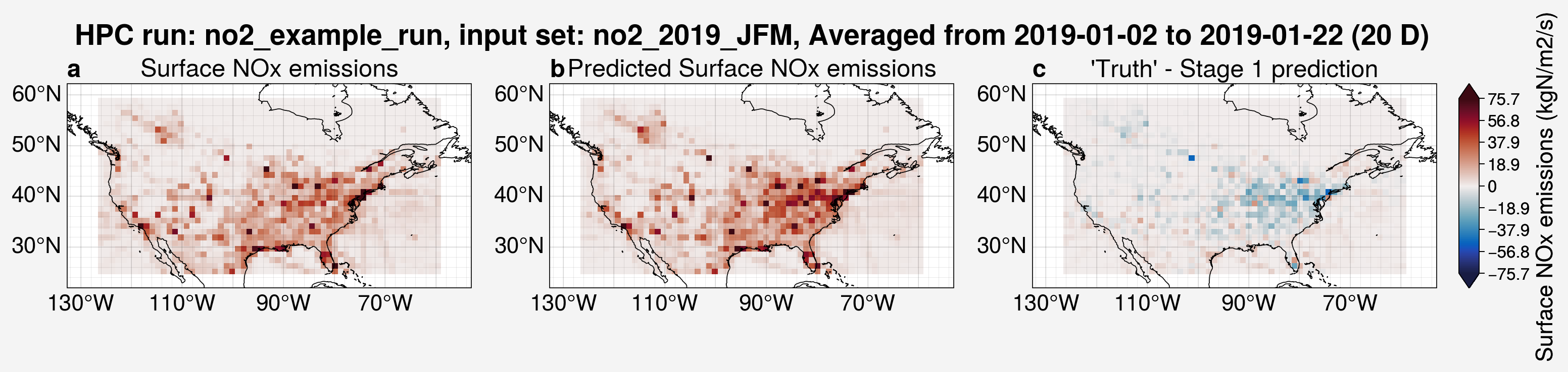
from unox.plotting import plot_run_analysis

this_plt = plot_run_analysis(
    no2_ex_uarr,
    start_date='2019-01-02',
    interval='20D',
    restrict_lat_lon_to='../datafiles/sample_data/nox_2019_t106_US.nc',
    add_corr_plots=False,
    stage1_only=True,
)
/home/docs/checkouts/readthedocs.org/user_builds/unox/envs/stable/lib/python3.9/site-packages/cartopy/mpl/geoaxes.py:403: UserWarning: The `map_projection` keyword argument is deprecated, use `projection` to instantiate a GeoAxes instead.
  warnings.warn("The `map_projection` keyword argument is "
/home/docs/checkouts/readthedocs.org/user_builds/unox/envs/stable/lib/python3.9/site-packages/cartopy/mpl/geoaxes.py:403: UserWarning: The `map_projection` keyword argument is deprecated, use `projection` to instantiate a GeoAxes instead.
  warnings.warn("The `map_projection` keyword argument is "
/home/docs/checkouts/readthedocs.org/user_builds/unox/envs/stable/lib/python3.9/site-packages/cartopy/mpl/geoaxes.py:403: UserWarning: The `map_projection` keyword argument is deprecated, use `projection` to instantiate a GeoAxes instead.
  warnings.warn("The `map_projection` keyword argument is "
As was mentioned above, the correlation plots can also be made on their own.
from unox.plotting import corr_plot

this_plt = corr_plot(
    no2_ex_uarr,
    is_predict=True,
    start_date='2019-02-01',
    interval='1M',
)
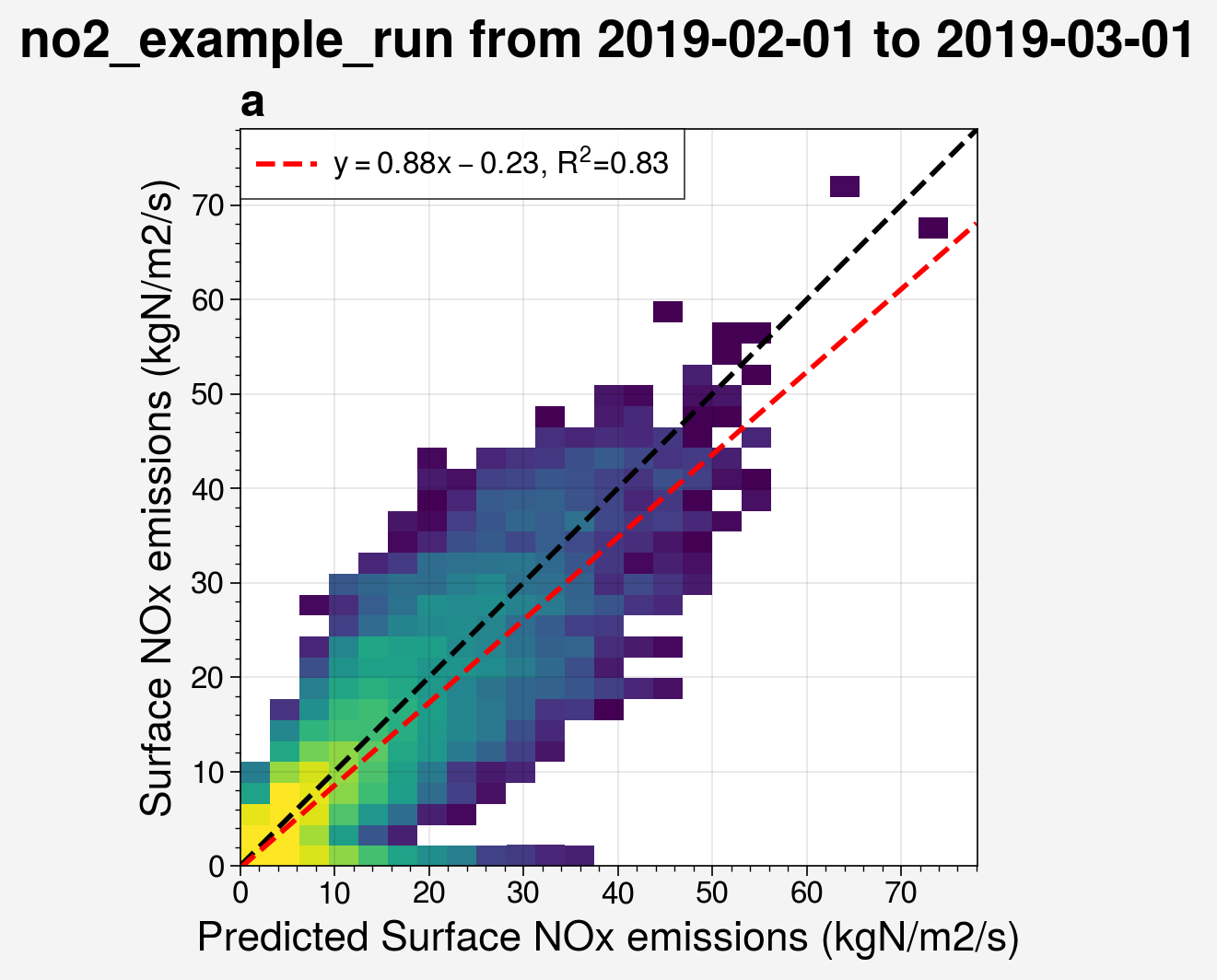
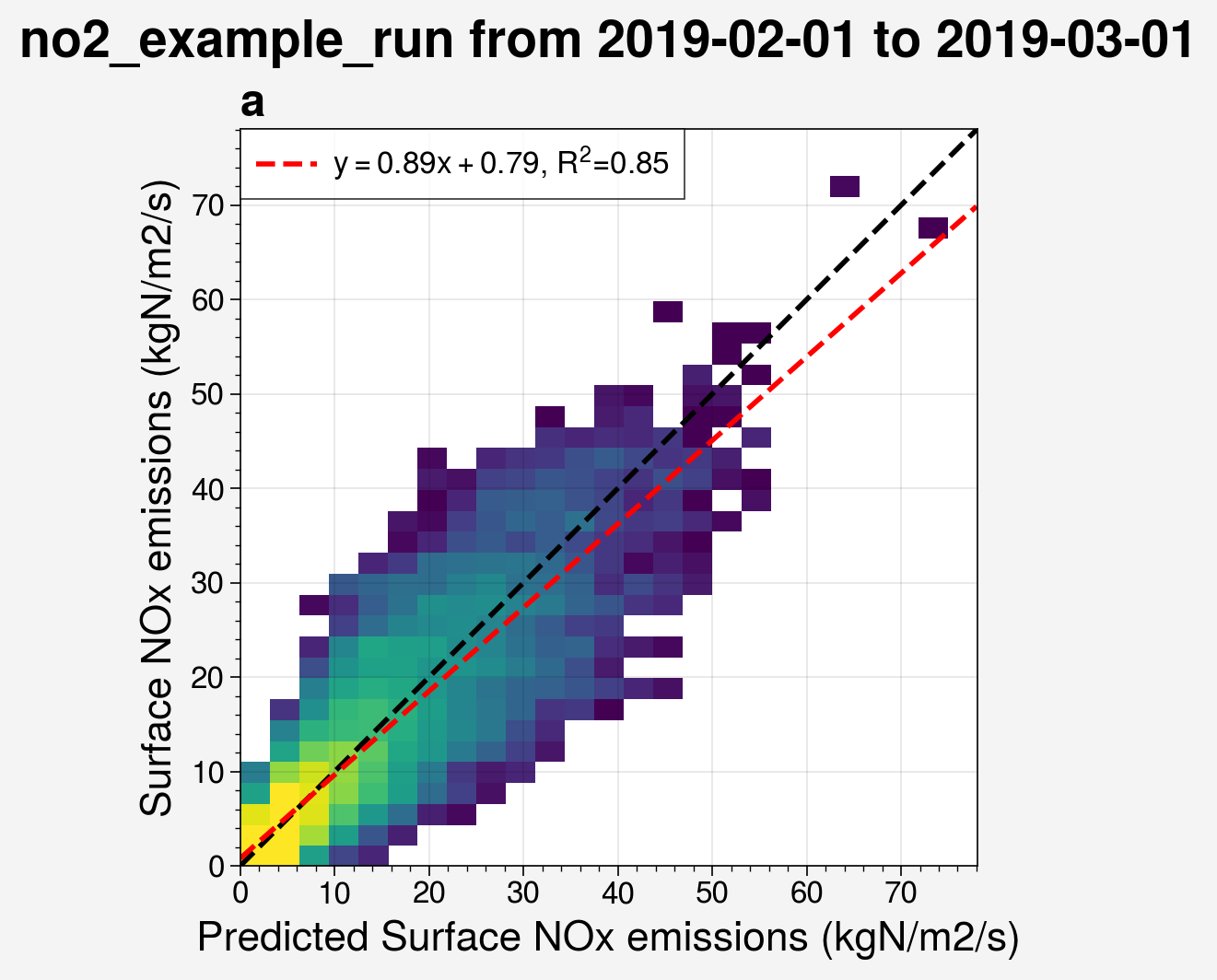
Restricting the latitude and longitude ranges has a noticeable effect on the correlation.
from unox.plotting import corr_plot

this_plt = corr_plot(
    no2_ex_uarr,
    is_predict=True,
    start_date='2019-02-01',
    interval='1M',
    restrict_lat_lon_to='../datafiles/sample_data/nox_2019_t106_US.nc',
)
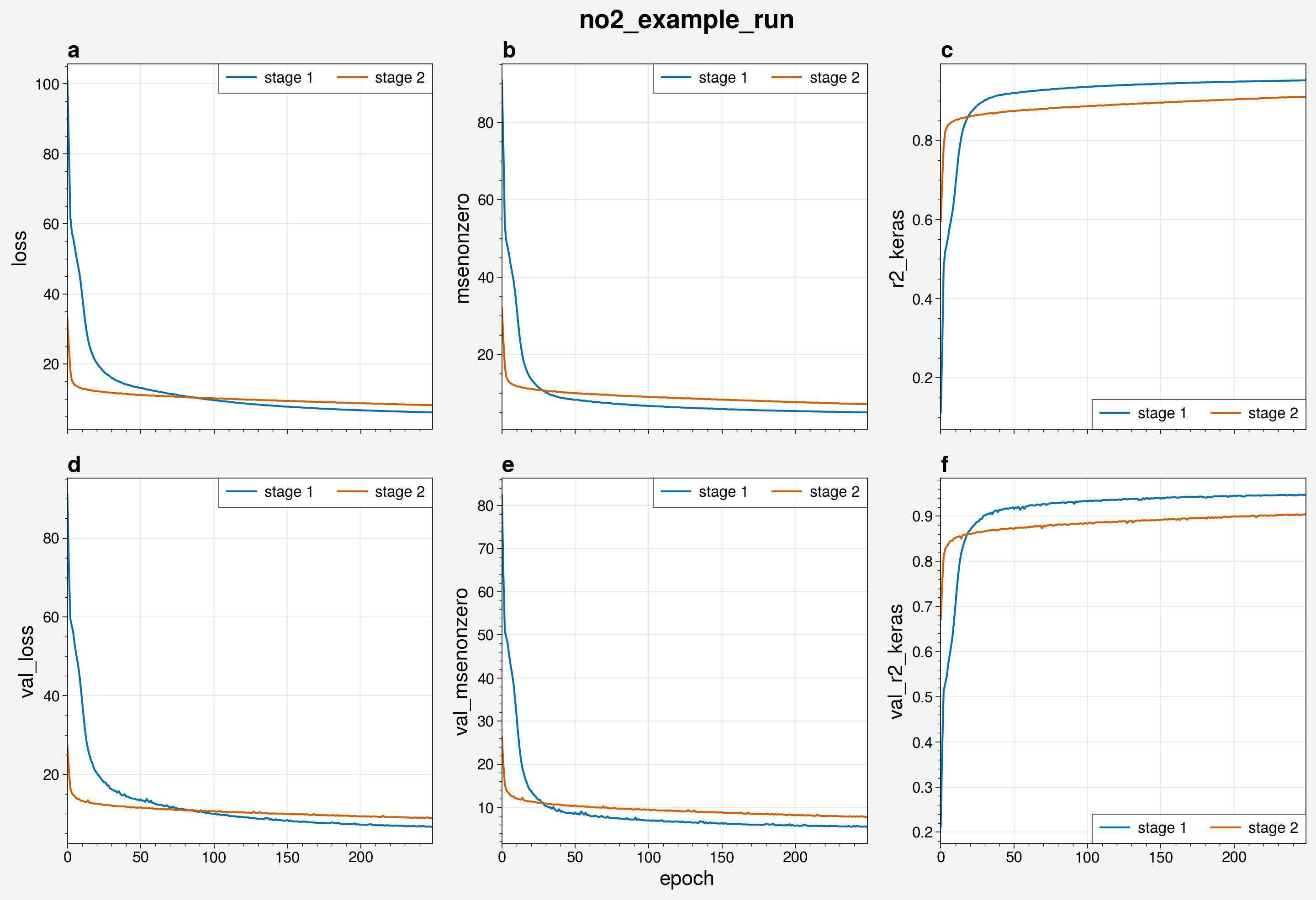
Several diagnostics are recorded into .csv files during a model run.
To view these diagnostics across the epochs of the model run, use the plot_epochs_logs() function.
from unox.plotting import plot_epochs_logs

this_plot = plot_epochs_logs(
    no2_ex_uarr,
    is_predict=True,
)