Running ensemble models
The documentation below describes how to run the U-net model with multiple ensemble members, then aggregate and analyze their results. This guide assumes you have followed the instructions on the Running the model to be familiar with submitting single model runs and, additionally, worked through the guide on Analyzing model output for a familiarity on how to plot different variables.
Contents
Introduction
The U-net model is stochastic, meaning that when running it multiple times, even with the exact same input and parameters, the results will always differ, if only slightly. This randomness is integral to how the U-net works, in contrast to models which are deterministic. If you were to run the model twice with slightly different input, it would be difficult to say whether any differences in the output would be due to those differences in input, or simply due to the expected variability of the randomness. To get an idea of what the spread of the stochastic variability is, we can run the U-net multiple times with the same configuration. This is called an ensemble run.
For this project, each ensemble run is submitted as a separate job to HPC, equivalent to following the procedure in the guide to Running the model. Below, we will work through an example of how to use the infrastructure in this code to avoid needing to submit each ensemble member separately. Afterwards, I’ll show how to use the plotting functions in this repository to analyze ensemble run outputs, both using the functions shown in Analyzing model output as well as functions specifically designed for plotting ensemble runs. Lastly, I’ll detail how ensemble runs can be used to assess a particular aspect of the model, in particular the regularizer function.
Running ensembles
Preparing ensemble runs
The preparation for ensemble runs is nearly identical to preparing a single model run, as described in the Running the model guide.
The key difference is that you will use the -e flag on the HPC_job_submit.sh script to tell it to create and submit multiple ensemble members at once.
Ensure that the input configuration file you want to use exists on HPC in inputfiles/_input_configs/.
For this example, I’ll use the default configuration file, inputfiles/_input_configs/sample_config.json, the contents of which are shown below.
{
    "input_set": "no2_2005-2020",
    "x_vars": [
        "no2",
        "no2_tm1",
        "u10",
        "v10",
        "blh",
        "sp",
        "skt",
        "t2m",
        "ssrd"
    ],
    "zfi_vars": [
    ],
    "lsm_vars": [
    ],
    "stage_2": true,
    "stage_2_cutoff": 2013,
    "n_epochs": 100,
    "split_year": 2019,
    "split_value": 0.9,
    "grid_size": [56, 120],
    "act_reg": "L1",
    "act_reg_factor": 1e-08
}
The attributes of this file are explained in Running the model.
Make sure your desired configuration file is on HPC.
For the example that follows, I’ll assume a custom configuration file called my_new_config.json.
Submitting ensemble runs
The HPC_job_submit.sh script includes a dedicated -e flag to handle ensemble submissions.
This single command automatically:
Creates the correct directory structure for all ensemble members
Copies the configuration file to each member’s directory
Submits all jobs to the HPC scheduler with appropriate naming
To submit 5 ensemble members with the job name no2_ens_test using the my_new_config input configuration, run this on HPC:
username@HPC: unox$ bash HPC_job_submit.sh -j no2_ens_test -i my_new_config -e 5
===== Begin HPC_job_submit.sh =====
-j, Name specified, using JOBNAME=no2_ens_test
-e, Ensemble size specified, using ENSEMBLE_SIZE=5
    Ensemble size is a valid integer from 1 to 99.
-i, Config files specified, using CONFIG_FILE=my_new_config
    Configuration file inputfiles/_input_configs/my_new_config.json found.
-t, No run type specified, using TYPE=test
    Using LAUNCHER=HPC_GPU_slurm.sh
-v, No version specified, using VERSION=1
-c, Using cluster: trillium
Creating directory for job no2_ens_test
    Creating subdirectories /01_no2_ens_test -- /05_no2_ens_test
Sending HPC notifications to email: <your_email@domain>
Submitted batch job 199501
Submitted batch job 199502
Submitted batch job 199503
Submitted batch job 199504
Submitted batch job 199505
The script creates this directory structure:
HPC_runs/
└── no2_ens_test/
    ├── ENSEMBLE_SIZE.txt          # Contains "5"
    ├── 01_no2_ens_test/
    │   └── input_config.json      # Copy of my_new_config.json
    ├── 02_no2_ens_test/
    │   └── input_config.json      # Same copy
    ├── 03_no2_ens_test/
    │   └── input_config.json      # Same copy
    ├── 04_no2_ens_test/
    │   └── input_config.json      # Same copy
    └── 05_no2_ens_test/
        └── input_config.json      # Same copy
Each subdirectory will accumulate output files (model, predictions, log files, etc.) as its corresponding job runs.
Monitoring ensemble jobs
To see all your ensemble jobs in the queue, use the mysq alias created in the Running the model guide (which amounts to squeue -u <username>) on HPC:
username@HPC: unox$ mysq
  JOBID        USER    ACCOUNT               NAME  ST  TIME_LEFT  PARTITION NODES  TRES_PER_NODE NODELIST (REASON)
 199501  <username>  def-dylan  no2_ens_test/01_n   R      58:32    compute     1     gres/gpu:1 trig0001 (None)
 199502  <username>  def-dylan  no2_ens_test/02_n   R      58:45    compute     1     gres/gpu:1 trig0002 (None)
 199503  <username>  def-dylan  no2_ens_test/03_n  PD         --    compute     1     gres/gpu:1 (Dependency)
 199504  <username>  def-dylan  no2_ens_test/04_n  PD         --    compute     1     gres/gpu:1 (QOSMaxJobsPerUserLimit)
 199505  <username>  def-dylan  no2_ens_test/05_n  PD         --    compute     1     gres/gpu:1 (QOSMaxJobsPerUserLimit)
Note that jobs may initially be in the PD (pending) state if there are queue limitations.
They will start as earlier jobs complete.
If you are running multiple ensembles at the same time, you can filter the output with grep to just show lines for one particular ensemble.
Note that this will not show the column headings.
username@HPC: unox$ mysq | grep no2_ens_test
 199501  <username>  def-dylan  no2_ens_test/01_n   R      58:32    compute     1     gres/gpu:1 trig0001 (None)
 199502  <username>  def-dylan  no2_ens_test/02_n   R      58:45    compute     1     gres/gpu:1 trig0002 (None)
 199503  <username>  def-dylan  no2_ens_test/03_n  PD         --    compute     1     gres/gpu:1 (Dependency)
 199504  <username>  def-dylan  no2_ens_test/04_n  PD         --    compute     1     gres/gpu:1 (QOSMaxJobsPerUserLimit)
 199505  <username>  def-dylan  no2_ens_test/05_n  PD         --    compute     1     gres/gpu:1 (QOSMaxJobsPerUserLimit)
As discussed in the Running the model guide, you can also monitor the jobs by opening their individual log files and checking your email.
Collecting ensemble results
Once all ensemble jobs have completed, transfer the entire ensemble output directory back to Animus by running the following command on Animus:
(env_name) username@animus-c:~/unox$ bash HPC_to_animus.sh -j -f no2_ens_test
-c, No cluster specified, defaulting to trillium
-j, Copying full HPC job directory for no2_ens_test from trillium to Animus
Directory ./HPC_runs/no2_ens_test does not exist, creating it.
Enter passphrase for key '/home/<username>/.ssh/<GH_id>':
(<username>@trillium.alliancecan.ca) Duo two-factor login for <username>

Enter a passcode or select one of the following options:

1. Duo Push to <mobile device>

Passcode or option (1-1): 1
Success. Logging you in...
Checking ./HPC_runs/no2_ens_test for ensemble predictions to combine...
    Found ./HPC_runs/no2_ens_test/ENSEMBLE_SIZE.txt
    Combining predictions from ensemble run for no2_ens_test
===== Begin combine_predictions.py =====
Current working directory: /home/<username>/unox
Given input arguments:
        argv[1], jobname:    no2_ens_test (no2_ens_test)
                 savedir:    HPC_runs/no2_ens_test/
All `input_config.json` files match across the 5 ensemble members.
        Saving `input_config.json` to HPC_runs/no2_ens_test/
All `output_metadata.json` files match across the 5 ensemble members.
        Saving `output_metadata.json` to HPC_runs/no2_ens_test/
Combining predictions from 5 ensemble members...
        Removing redundant file: HPC_runs/no2_ens_test/01_no2_ens_test/predictions.nc
        Removing redundant file: HPC_runs/no2_ens_test/02_no2_ens_test/predictions.nc
        Removing redundant file: HPC_runs/no2_ens_test/03_no2_ens_test/predictions.nc
        Removing redundant file: HPC_runs/no2_ens_test/04_no2_ens_test/predictions.nc
        Removing redundant file: HPC_runs/no2_ens_test/05_no2_ens_test/predictions.nc
===== End combine_predictions.py =====

Checking ./HPC_runs/no2_ens_test/01_no2_ens_test for ensemble predictions to combine...
    No predictions within ./HPC_runs/no2_ens_test/01_no2_ens_test to combine
Checking ./HPC_runs/no2_ens_test/02_no2_ens_test for ensemble predictions to combine...
    No predictions within ./HPC_runs/no2_ens_test/02_no2_ens_test to combine
Checking ./HPC_runs/no2_ens_test/03_no2_ens_test for ensemble predictions to combine...
    No predictions within ./HPC_runs/no2_ens_test/03_no2_ens_test to combine
Checking ./HPC_runs/no2_ens_test/04_no2_ens_test for ensemble predictions to combine...
    No predictions within ./HPC_runs/no2_ens_test/04_no2_ens_test to combine
Checking ./HPC_runs/no2_ens_test/05_no2_ens_test for ensemble predictions to combine...
    No predictions within ./HPC_runs/no2_ens_test/05_no2_ens_test to combine
Completed file transfer to Animus
This single command transfers the entire HPC_runs/no2_ens_test/ directory with all 5 ensemble members and their outputs back to Animus, then automatically runs combine_predictions.py.
That Python script will find all the individual .nc files from each ensemble member and combine them together.
During that process, the prediction variable names will have their ensemble number appended to them such that you can easily distinguish the predictions of each ensemble member later.
Finally, it deletes the now-redundant .nc files in each ensemble member’s directory.
This will save on the storage space required on Animus.
Analyzing ensemble output
With ensemble outputs on Animus, you can visualize and compare predictions across members to understand uncertainty and robustness. This section demonstrates how to use the plotting functions provided in this repository to analyze ensemble run outputs, following similar approaches as described in the Analyzing model output guide.
Exploring an ensemble dataset
To see what is in an ensemble run predictions dataset, you can load it as a uarray object and call the .xr attribute.
Below is a text representation of the output.
However, if the below python commands are executed in a Jupyter Notebook cell on Animus, the structure becomes interactive, allowing for more exploration (see Analysis).
from unox.HPC.data0.dataset import uarray

my_ensemble = uarray('no2_ens_test', is_predict=True)
my_ensemble.xr
<xarray.Dataset> Size: 196MB
Dimensions:         (time: 728, lat: 56, lon: 120)
Coordinates:
  * time            (time) object 6kB 2019-01-02 00:00:00 ... 2020-12-31 00:0...
  * lat             (lat) float32 224B 11.78 12.9 14.02 ... 71.21 72.34 73.46
  * lon             (lon) float32 480B -174.4 -173.2 -172.1 ... -41.62 -40.5
Data variables:
    nox_pred_01     (time, lat, lon) float32 20MB ...
    nox_pred_s2_01  (time, lat, lon) float32 20MB ...
    nox_pred_02     (time, lat, lon) float32 20MB ...
    nox_pred_s2_02  (time, lat, lon) float32 20MB ...
    nox_pred_03     (time, lat, lon) float32 20MB ...
    nox_pred_s2_03  (time, lat, lon) float32 20MB ...
    nox_pred_04     (time, lat, lon) float32 20MB ...
    nox_pred_s2_04  (time, lat, lon) float32 20MB ...
    nox_pred_05     (time, lat, lon) float32 20MB ...
    nox_pred_s2_05  (time, lat, lon) float32 20MB ...
Attributes: (12/19)
    description:        Predicted Surface NOx emissions using a U-net model
    modification_date:  2026-03-09 15:21:02
    y_var:              nox
    input_set:          no2_2005-2020
    config_path:        HPC_runs/no2_ens_test/01_no2_ens_test/input_config.json
    config_dict:        {'input_set': 'no2_2005-2020', 'x_vars': ['no2', 'no2...
    ...                 ...
    data_dir:           /data/high_res
    chemra_path:        emacdonald/unet/datafiles/TROPESS/TROPESS_reanalysis_...
    insitu_path:        US_EPA/NO2/daily_NO2/daily_42602_
    era5_path:          ERA5concatenated
    stages:             [1 2]
    ensemble_size:      5
This is similar to a predictions.nc file that was not an ensemble run.
The difference is that, with an ensemble, there is a separate data variable for each output (stage 1 and/or 2) for each ensemble member.
Each data variable has it’s ensemble member ID appended to its name.
For example, the predicted NOx for stage 2 for ensemble member 1 has the name nox_pred_s2_01.
Plotting ensemble members
Most plotting functions will accept the argument ens_mem to specify which ensemble member to plot.
This allows you to make plots for each individual ensemble member in the same way as non-ensemble runs, no need to append the ensemble member ID to the name of the variable to plot.
from unox.plotting import plot_var_maps

this_plt = plot_var_maps(
    'no2_ens_test',
    ens_mem=1,
    is_predict=True,
    vars=['nox_pred', 'nox_pred_s2'],
    start_date='2019-01-01',
    interval='1Y',
)
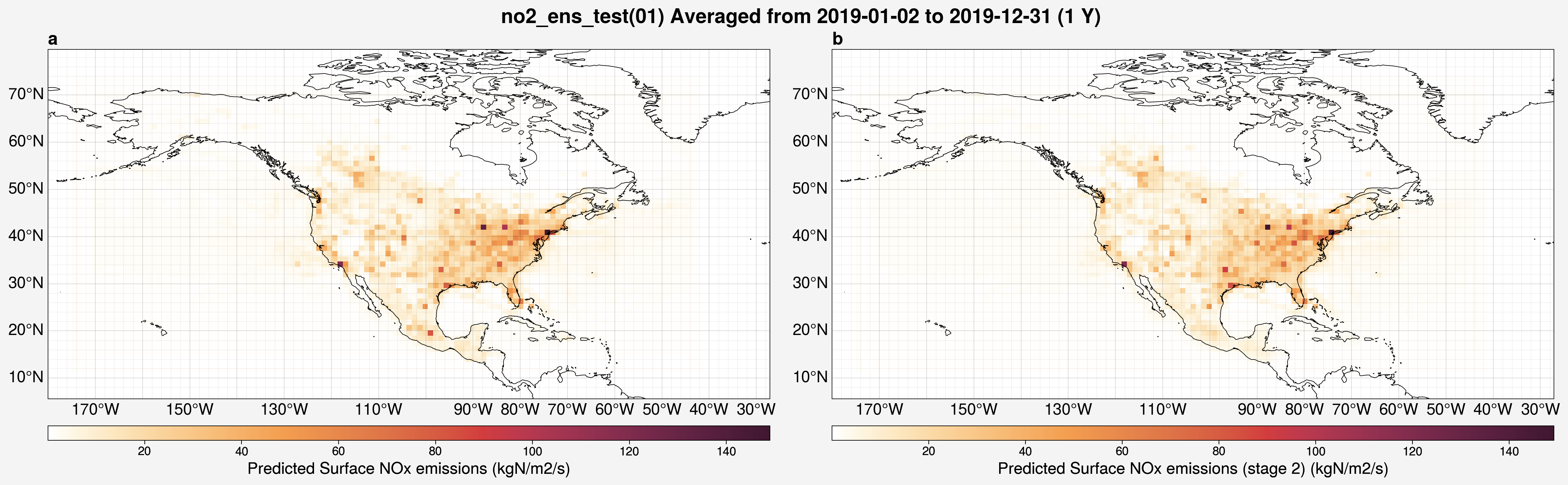
The ensemble member ID will be automatically added to the title.
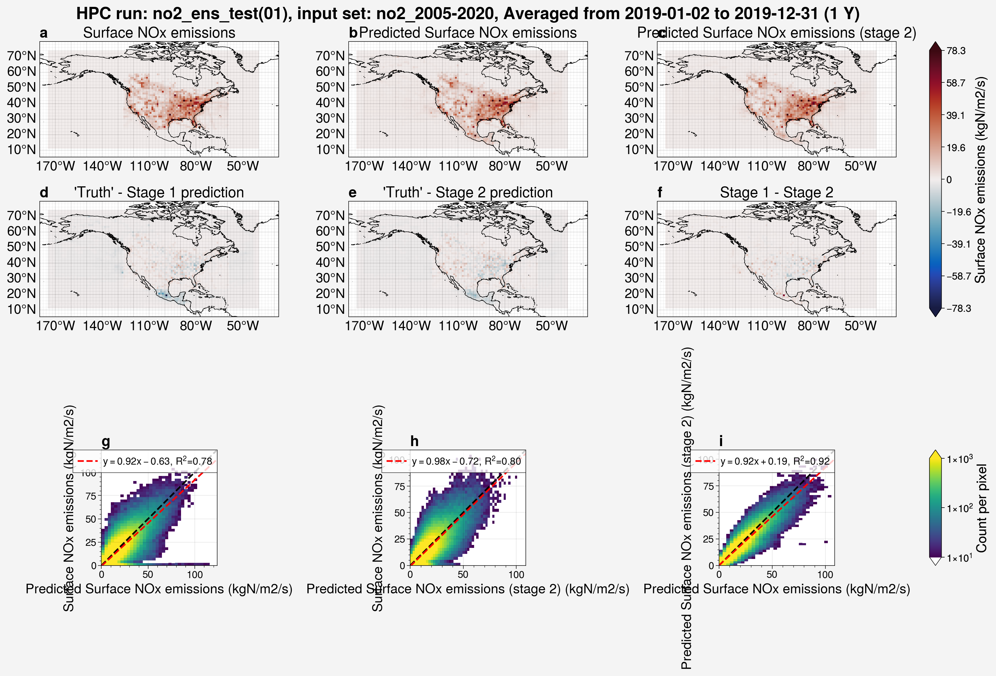
Similarly, the results of a model run can be quickly visualized using the plot_run_analysis() function for a particular ensemble member.
from unox.plotting import plot_run_analysis

this_plt = plot_run_analysis(
    'no2_ens_test',
    ens_mem=1,
    start_date='2019-01-01',
)
Box and whisker plots
The major benefit of running an ensemble is to be able to view the statistical spread in performance among the members. Box and whisker plots provide a compact way to visualize these distributions.
from unox.plotting import plot_BaW

this_plot = plot_BaW(
    ['R2', 'RMSE'],
    'no2_example_ens_run',
    ds_kwargs=[
        {
            'is_predict': True,
            'start_date': '2019-01-02',
            'interval': '1Y',
        },
    ]
)
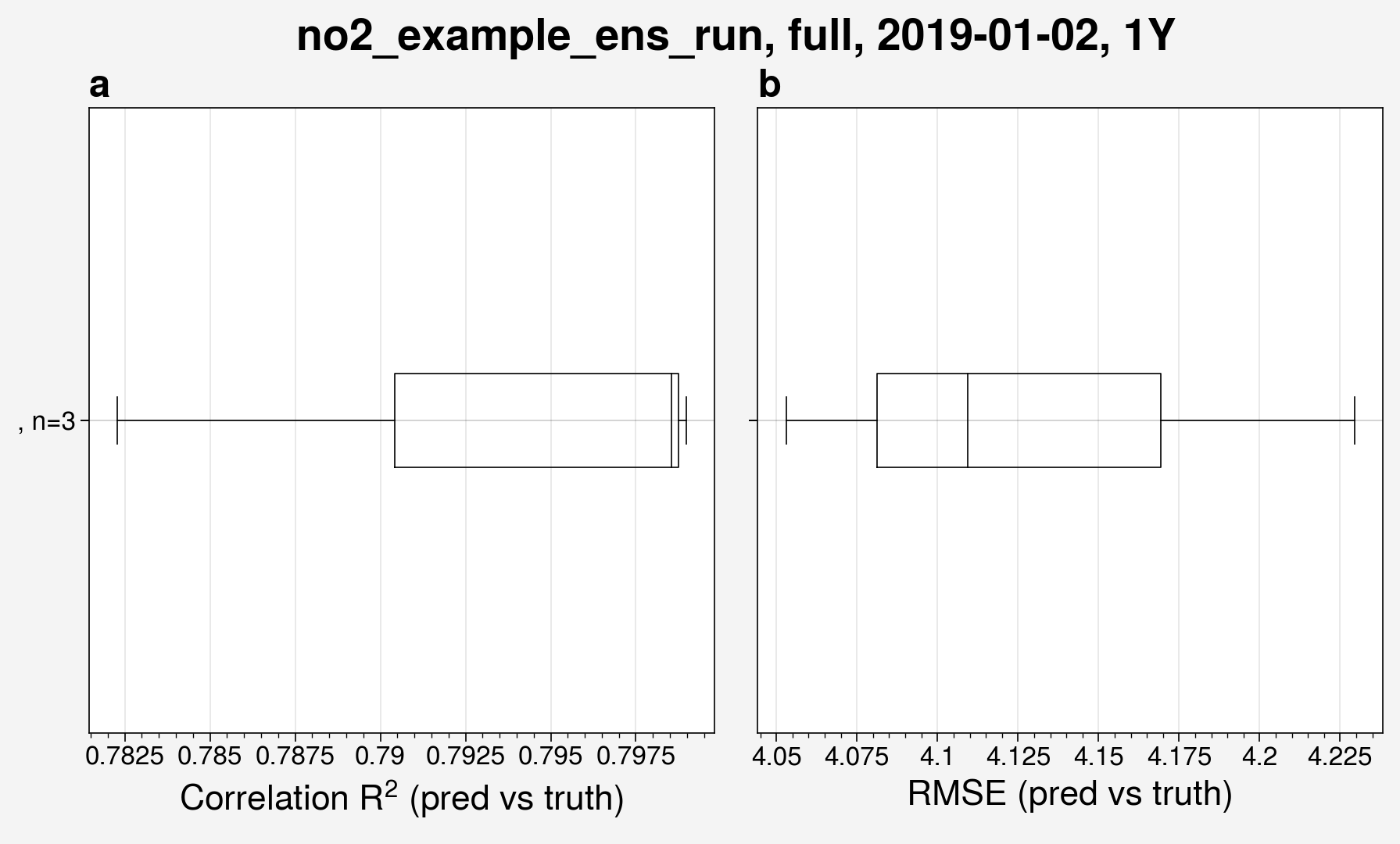
This shows the spread in \(R^2\) and root mean squared error (RMSE) for the ensemble run. Note that the box and whisker function will create a plot regardless of how many ensemble members there are. Use caution when analyzing box and whisker plots for ensembles with 3 or fewer members.
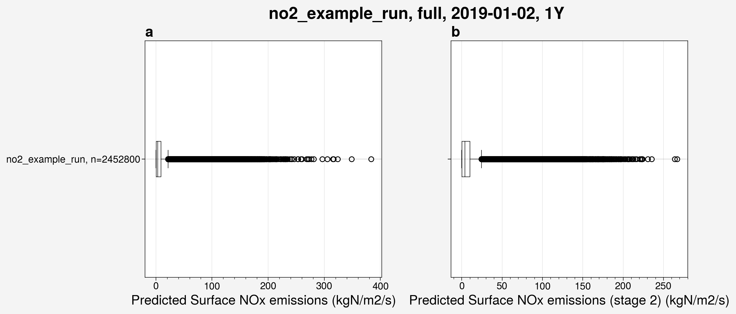
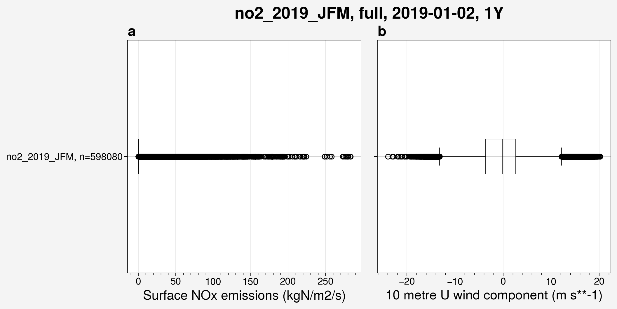
Box and whisker plots can also be used to visualize the spread in any variable, whether from prediction datasets or input files.
from unox.plotting import plot_BaW

this_plot = plot_BaW(
    ['nox_pred', 'nox_pred_s2'],
    'no2_example_run',
    ds_kwargs=[
        {
            'is_predict': True,
            'start_date': '2019-01-02',
            'interval': '1Y',
        },
    ],
)
from unox.plotting import plot_BaW

this_plot = plot_BaW(
    ['nox', 'u10'],
    'no2_2019_JFM',
    ds_kwargs=[
        {
            'is_input_set': True,
            'start_date': '2019-01-02',
            'interval': '1Y',
        },
    ],
)
Example: Assessing impact of regularizers
Ensemble runs are particularly useful for assessing the impact of specific model components or hyperparameters on prediction robustness and uncertainty. In this section, we demonstrate how to use ensemble runs to systematically evaluate the effect on model performance of using a regularizer.
What is a regularizer?
Regularizers are techniques used during neural network training to prevent overfitting and improve generalization. A common regularization method is called L1/L2 regularization, which involves adding penalty terms to the loss function based on weight magnitudes. This can help prevent erroneous values in the predictions, especially in regions where values close to zero are expected.
In the Keras documentation of regularizers, they mention that three different types of regularizers are available for use:
kernel_regularizer: Regularizer to apply a penalty on the layer’s kernel.
bias_regularizer: Regularizer to apply a penalty on the layer’s bias.
activity_regularizer: Regularizer to apply a penalty on the layer’s output.
You can also look at the keras.regularizers source code.
As the goal is to prevent the output of the model to have erroneous non-zero values, I decided to use the activity regularizer.
I applied this to all every Conv2D, Conv2DTranspose, and LSTM layer in the Unet, as can be seen in the src/unox/HPC/model/core.py file.
I have implemented 4 different options for a regularizer to use:
L1L2L1L2None
When using a regularizer, the chosen function takes in a float parameter which is the “regularization factor.”
In examples, I see most often this is a value like 0.01 or 0.03, but I’ve also seen up to 2.0.
Below, I will examine the effect of choosing different values of this factor.
By running multiple ensemble members with and without specific regularizers, you can quantitatively assess:
Whether a regularizer reduces ensemble uncertainty.
If the regularizer improves spatial consistency of predictions.
How the regularizer affects prediction accuracy at different locations.
Configuring regularizer ensemble runs
To compare the impact of regularizers, we can create multiple input configuration files that differ only in regularization settings. For example:
Configuration 0: Without a regularizer (config_ens_reg0.json):
{
    "input_set": "no2_2005-2020",
    "x_vars": [
        "no2",
        "no2_tm1",
        "u10",
        "v10",
        "blh",
        "sp",
        "skt",
        "t2m",
        "ssrd"
    ],
    "zfi_vars": [
    ],
    "lsm_vars": [
    ],
    "stage_2": true,
    "stage_2_cutoff": 2013,
    "n_epochs": 100,
    "split_year": 2019,
    "split_value": 0.9,
    "grid_size": [56, 120],
    "act_reg": "None",
    "act_reg_factor": 1
}
Configuration 1: With L1 regularizer and a factor of \(1\times10^{-5}\) (config_ens_reg1.json):
{
    "input_set": "no2_2005-2020",
    "x_vars": [
        "no2",
        "no2_tm1",
        "u10",
        "v10",
        "blh",
        "sp",
        "skt",
        "t2m",
        "ssrd"
    ],
    "zfi_vars": [
    ],
    "lsm_vars": [
    ],
    "stage_2": true,
    "stage_2_cutoff": 2013,
    "n_epochs": 100,
    "split_year": 2019,
    "split_value": 0.9,
    "grid_size": [56, 120],
    "act_reg": "L1",
    "act_reg_factor": 1e-05
}
With both of these configuration files on HPC in inputfiles/_input_configs/, you can submit two separate ensemble runs:
username@HPC: unox$ bash HPC_job_submit.sh -j ens_reg0 -i config_ens_reg0 -e 5
username@HPC: unox$ bash HPC_job_submit.sh -j ens_reg1 -i config_ens_reg1 -e 5
For this example, I submitted 5 more ensemble runs, each with 5 members, using regularizer factors each order of magnitude from \(1\times10^{-6}\) to \(1\times10^{-10}\).
Plotting regularizer impact
Once all ensemble runs are complete and transferred to Animus, you can compare predictions on Animus. First, we can take a look at the results for particular ensemble members in select ensemble runs.
from unox.plotting import plot_run_analysis

var_plots = plot_run_analysis(
    'ens_reg0',
    ens_mem=1,
)
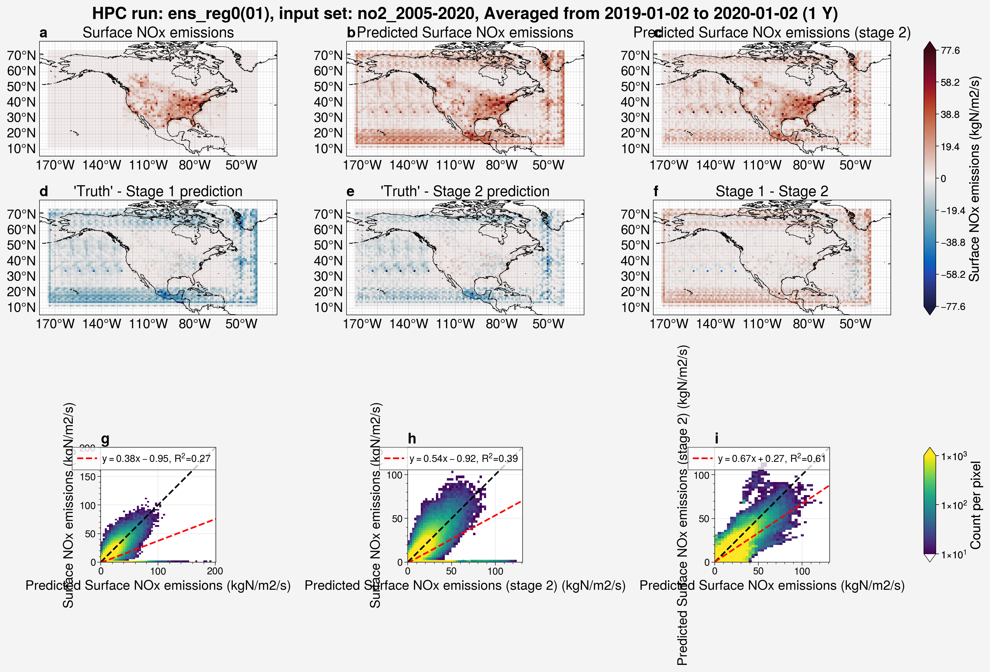
Above, we can see that running with no regularizer results in artifacts in the predictions, notably non-zero values around the edges of the domain and over the ocean. This is very similar to the result when using a regularizer with a factor that is too small, in this case \(1\times 10^{-10}\).
from unox.plotting import plot_run_analysis

var_plots = plot_run_analysis(
    'ens_reg1',
    ens_mem=1,
)
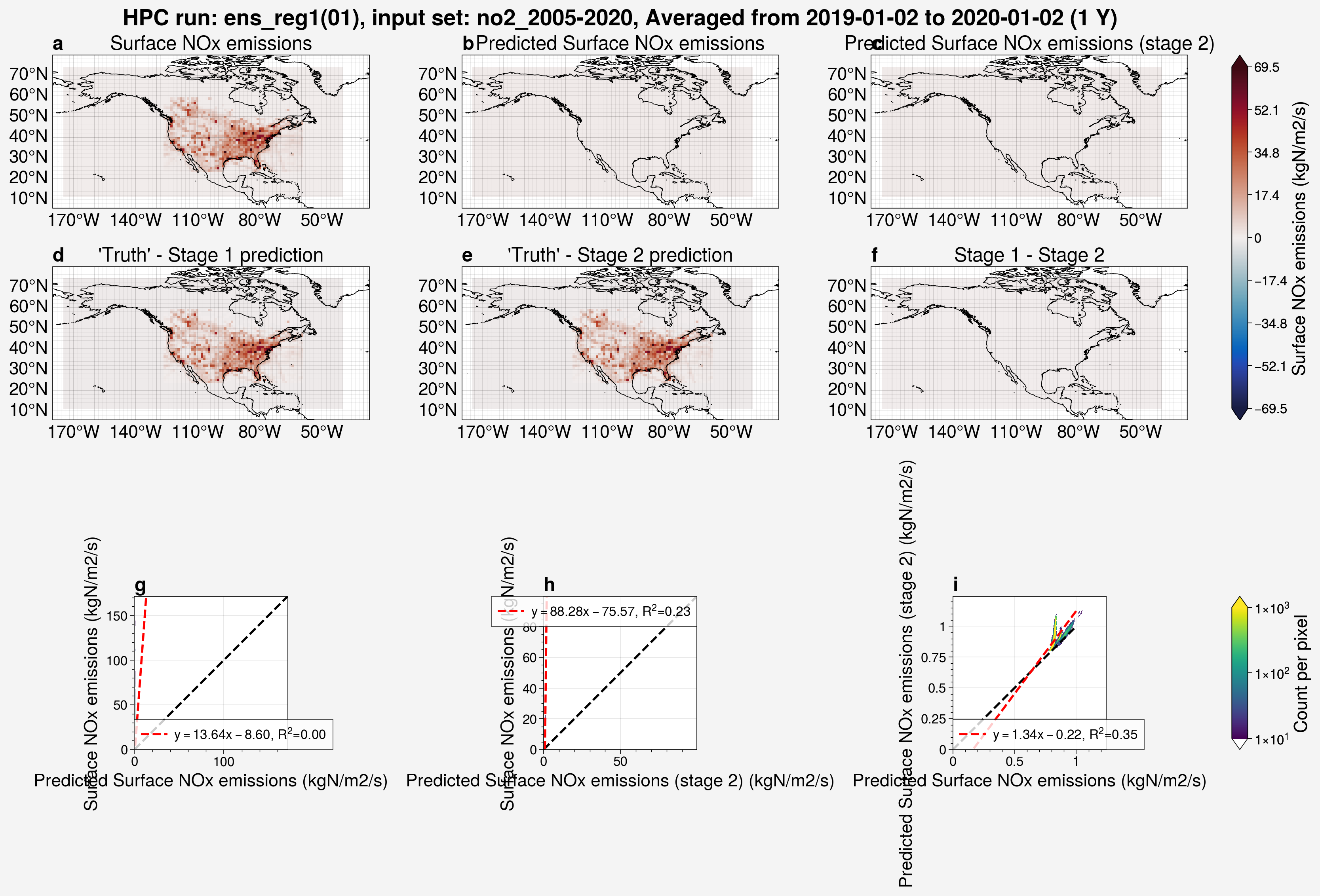
In the above example, we can see that the regularizer factor was set too high at \(1\times 10^{-5}\) and resulted in all the predictions being far too small across the entire domain.
from unox.plotting import plot_run_analysis

var_plots = plot_run_analysis(
    'ens_reg4',
    ens_mem=1,
)
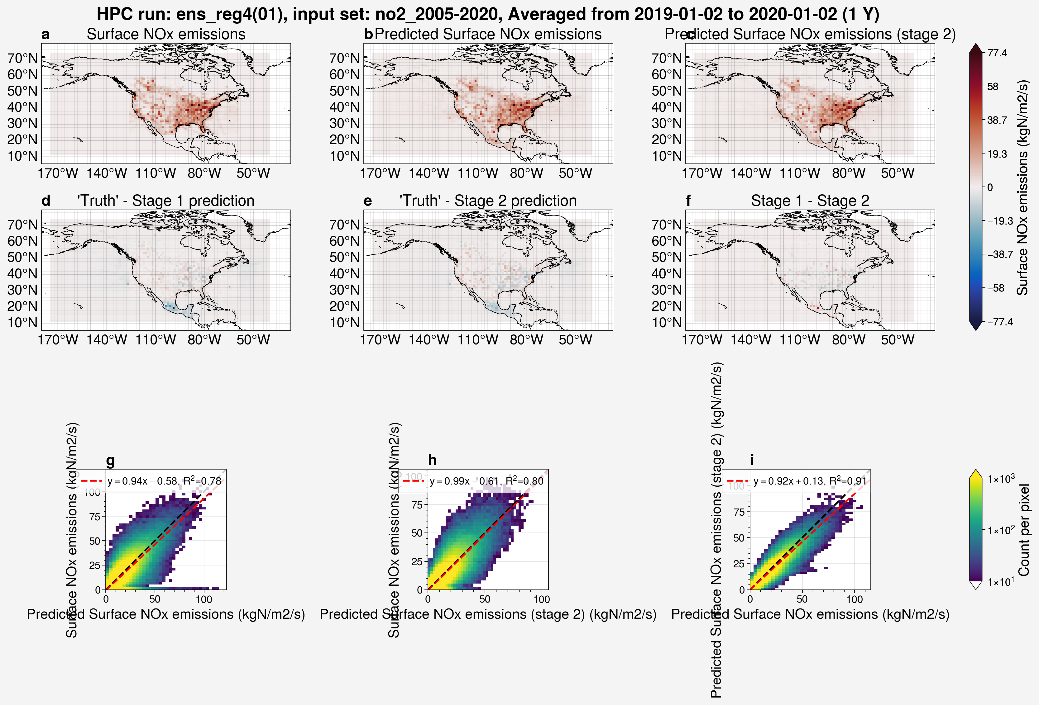
Here, we can see in the plot above that, with a regularizer factor of \(1\times10^{-8}\), the model does a much better job at predicting the output.
To see the statistical spread of all these ensembles at once, we can make a box and whisker plot.
Below, I have used the label_with attribute to specify that I want the labels of each ensemble run to be the activity regularizer used (act_reg) and the regularizer factor used in the activity regularizer (act_reg_factor).
The label_with list can contain any key names from the configuration file.
from unox.plotting import plot_BaW

this_plot = plot_BaW(
    ['R2', 'RMSE'],
    ['ens_reg0', 'ens_reg1', 'ens_reg2', 'ens_reg3', 'ens_reg4', 'ens_reg5', 'ens_reg6'],
    ds_kwargs=[
        {
            'is_predict': True,
            'start_date': '2019-01-02',
            'interval': '1Y',
        },
    ],
    label_with=['act_reg', 'act_reg_factor']
)
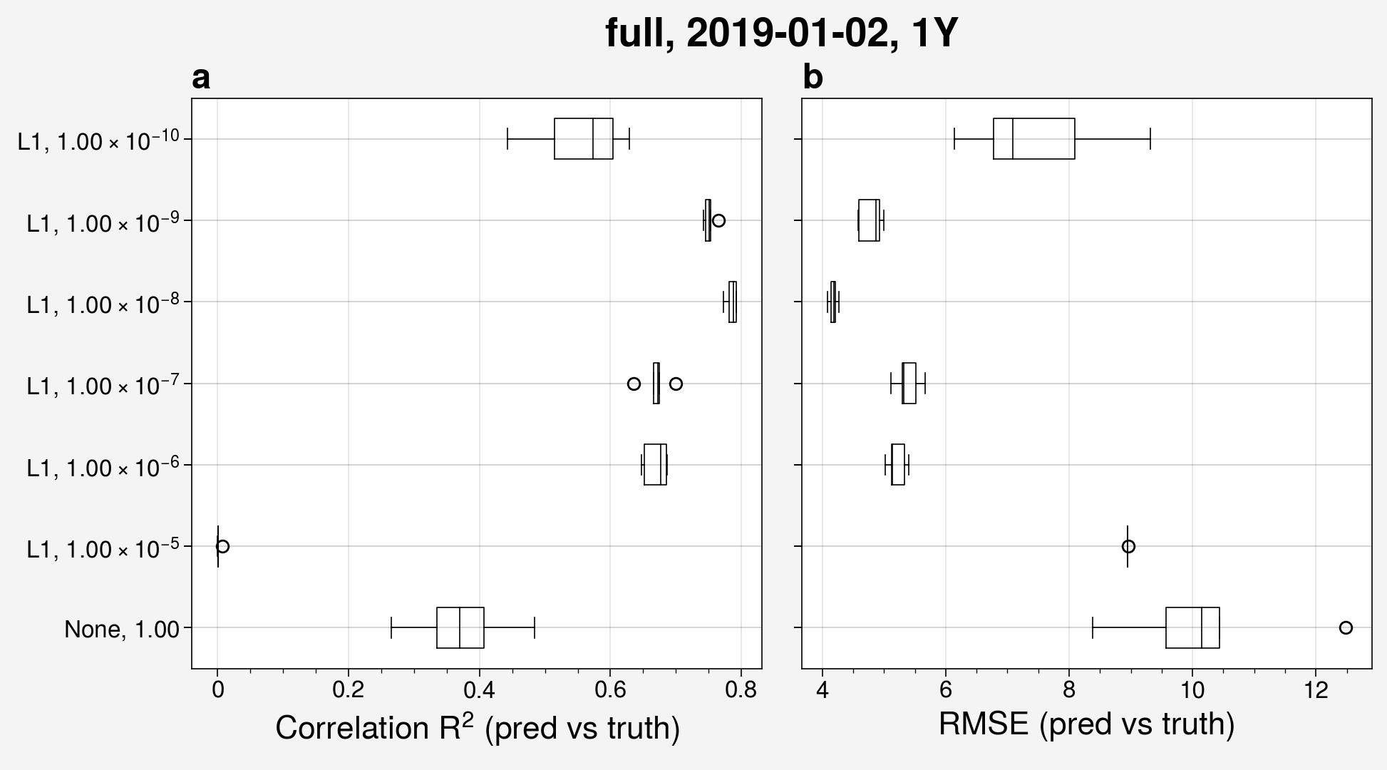
Here, we can see that using a factor of \(1\times10^{-8}\) improves the model the most out of the factors used across the ensemble runs.
We can also make the same plot, but restrict the latitude and longitude extent to be just over the continental United States.
from unox.plotting import plot_BaW

this_plot = plot_BaW(
    ['R2', 'RMSE'],
    ['ens_reg0', 'ens_reg1', 'ens_reg2', 'ens_reg3', 'ens_reg4', 'ens_reg5', 'ens_reg6'],
    ds_kwargs=[
        {
            'is_predict': True,
            'start_date': '2019-01-02',
            'interval': '1Y',
            'restrict_lat_lon_to': 'datafiles/sample_data/nox_2019_t106_US.nc',
        },
    ],
    label_with=['act_reg', 'act_reg_factor']
)
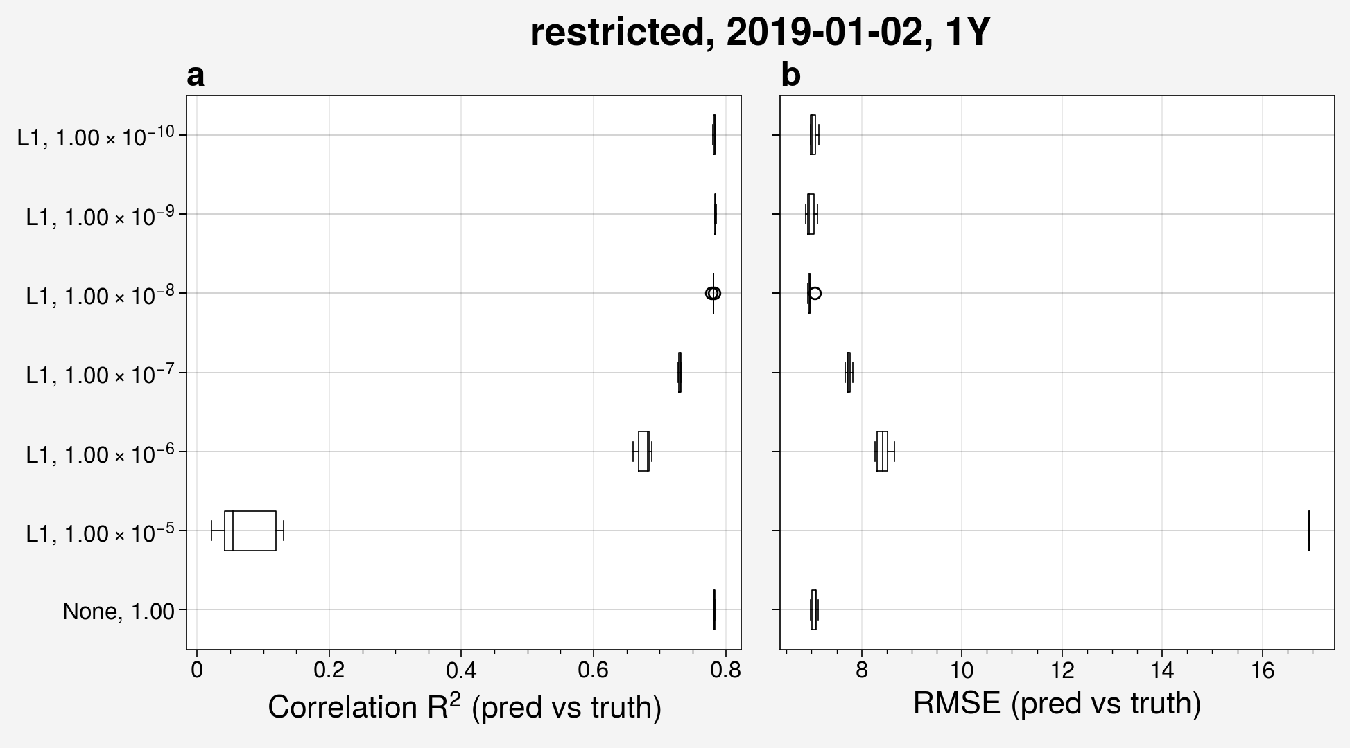
I have found similar results for using the L2 function in the regularizer.